library(tidyverse)
library(ggplot2)
library(summarytools)
library(lubridate)

knitr::opts_chunk$set(echo = TRUE, warning=FALSE, message=FALSE)
Challenge 7
challenge_7
hotel_bookings
Aleacia Messiah
tidyverse
ggplot2
summarytools
lubridate
Visualizing Multiple Dimensions
Challenge Overview
Today’s challenge is to:
- read in a data set, and describe the data set using both words and any supporting information (e.g., tables, etc)
- tidy data (as needed, including sanity checks)
- mutate variables as needed (including sanity checks)
- Recreate at least two graphs from previous exercises, but introduce at least one additional dimension that you omitted before using ggplot functionality (color, shape, line, facet, etc) The goal is not to create unneeded chart ink (Tufte), but to concisely capture variation in additional dimensions that were collapsed in your earlier 2 or 3 dimensional graphs.
- Explain why you choose the specific graph type
- If you haven’t tried in previous weeks, work this week to make your graphs “publication” ready with titles, captions, and pretty axis labels and other viewer-friendly features
R Graph Gallery is a good starting point for thinking about what information is conveyed in standard graph types, and includes example R code. And anyone not familiar with Edward Tufte should check out his fantastic books and courses on data visualization.
(be sure to only include the category tags for the data you use!)
Read in data
Read in one (or more) of the following datasets, using the correct R package and command.
eggs ⭐
abc_poll ⭐⭐
australian_marriage ⭐⭐
hotel_bookings ⭐⭐⭐
air_bnb ⭐⭐⭐
us_hh ⭐⭐⭐⭐
faostat ⭐⭐⭐⭐⭐
NotePlease note that since this challenge is to recreate my graphs from previous challenges, I will be using the same dataset (hotel_bookings.csv) to recreate my graphs from Challenge 6, hence why my code for reading in, tidying, and mutating the dataset will also be the same.
# read in hotel data
hotel_orig <- read_csv("_data/hotel_bookings.csv")
# view hotel data
hotel_orig
# A tibble: 119,390 × 32
hotel is_ca…¹ lead_…² arriv…³ arriv…⁴ arriv…⁵ arriv…⁶ stays…⁷ stays…⁸ adults
<chr> <dbl> <dbl> <dbl> <chr> <dbl> <dbl> <dbl> <dbl> <dbl>
1 Resor… 0 342 2015 July 27 1 0 0 2
2 Resor… 0 737 2015 July 27 1 0 0 2
3 Resor… 0 7 2015 July 27 1 0 1 1
4 Resor… 0 13 2015 July 27 1 0 1 1
5 Resor… 0 14 2015 July 27 1 0 2 2
6 Resor… 0 14 2015 July 27 1 0 2 2
7 Resor… 0 0 2015 July 27 1 0 2 2
8 Resor… 0 9 2015 July 27 1 0 2 2
9 Resor… 1 85 2015 July 27 1 0 3 2
10 Resor… 1 75 2015 July 27 1 0 3 2
# … with 119,380 more rows, 22 more variables: children <dbl>, babies <dbl>,
# meal <chr>, country <chr>, market_segment <chr>,
# distribution_channel <chr>, is_repeated_guest <dbl>,
# previous_cancellations <dbl>, previous_bookings_not_canceled <dbl>,
# reserved_room_type <chr>, assigned_room_type <chr>, booking_changes <dbl>,
# deposit_type <chr>, agent <chr>, company <chr>, days_in_waiting_list <dbl>,
# customer_type <chr>, adr <dbl>, required_car_parking_spaces <dbl>, …# view summary of hotel data
dfSummary(hotel_orig)Data Frame Summary
hotel_orig
Dimensions: 119390 x 32
Duplicates: 31994
-----------------------------------------------------------------------------------------------------------------------------------
No Variable Stats / Values Freqs (% of Valid) Graph Valid Missing
---- -------------------------------- -------------------------- ---------------------- ---------------------- ---------- ---------
1 hotel 1. City Hotel 79330 (66.4%) IIIIIIIIIIIII 119390 0
[character] 2. Resort Hotel 40060 (33.6%) IIIIII (100.0%) (0.0%)
2 is_canceled Min : 0 0 : 75166 (63.0%) IIIIIIIIIIII 119390 0
[numeric] Mean : 0.4 1 : 44224 (37.0%) IIIIIII (100.0%) (0.0%)
Max : 1
3 lead_time Mean (sd) : 104 (106.9) 479 distinct values : 119390 0
[numeric] min < med < max: : (100.0%) (0.0%)
0 < 69 < 737 :
IQR (CV) : 142 (1) : : .
: : : . .
4 arrival_date_year Mean (sd) : 2016.2 (0.7) 2015 : 21996 (18.4%) III 119390 0
[numeric] min < med < max: 2016 : 56707 (47.5%) IIIIIIIII (100.0%) (0.0%)
2015 < 2016 < 2017 2017 : 40687 (34.1%) IIIIII
IQR (CV) : 1 (0)
5 arrival_date_month 1. August 13877 (11.6%) II 119390 0
[character] 2. July 12661 (10.6%) II (100.0%) (0.0%)
3. May 11791 ( 9.9%) I
4. October 11160 ( 9.3%) I
5. April 11089 ( 9.3%) I
6. June 10939 ( 9.2%) I
7. September 10508 ( 8.8%) I
8. March 9794 ( 8.2%) I
9. February 8068 ( 6.8%) I
10. November 6794 ( 5.7%) I
[ 2 others ] 12709 (10.6%) II
6 arrival_date_week_number Mean (sd) : 27.2 (13.6) 53 distinct values . : . . . 119390 0
[numeric] min < med < max: . : : : : : : (100.0%) (0.0%)
1 < 28 < 53 . : : : : : : : : :
IQR (CV) : 22 (0.5) : : : : : : : : : :
: : : : : : : : : :
7 arrival_date_day_of_month Mean (sd) : 15.8 (8.8) 31 distinct values : 119390 0
[numeric] min < med < max: : : : . : : . : : (100.0%) (0.0%)
1 < 16 < 31 : : : : : : : : : :
IQR (CV) : 15 (0.6) : : : : : : : : : :
: : : : : : : : : :
8 stays_in_weekend_nights Mean (sd) : 0.9 (1) 17 distinct values : 119390 0
[numeric] min < med < max: : (100.0%) (0.0%)
0 < 1 < 19 :
IQR (CV) : 2 (1.1) : :
: :
9 stays_in_week_nights Mean (sd) : 2.5 (1.9) 35 distinct values : 119390 0
[numeric] min < med < max: : (100.0%) (0.0%)
0 < 2 < 50 :
IQR (CV) : 2 (0.8) :
:
10 adults Mean (sd) : 1.9 (0.6) 14 distinct values : 119390 0
[numeric] min < med < max: : (100.0%) (0.0%)
0 < 2 < 55 :
IQR (CV) : 0 (0.3) :
:
11 children Mean (sd) : 0.1 (0.4) 0 : 110796 (92.8%) IIIIIIIIIIIIIIIIII 119386 4
[numeric] min < med < max: 1 : 4861 ( 4.1%) (100.0%) (0.0%)
0 < 0 < 10 2 : 3652 ( 3.1%)
IQR (CV) : 0 (3.8) 3 : 76 ( 0.1%)
10 : 1 ( 0.0%)
12 babies Mean (sd) : 0 (0.1) 0 : 118473 (99.2%) IIIIIIIIIIIIIIIIIII 119390 0
[numeric] min < med < max: 1 : 900 ( 0.8%) (100.0%) (0.0%)
0 < 0 < 10 2 : 15 ( 0.0%)
IQR (CV) : 0 (12.3) 9 : 1 ( 0.0%)
10 : 1 ( 0.0%)
13 meal 1. BB 92310 (77.3%) IIIIIIIIIIIIIII 119390 0
[character] 2. FB 798 ( 0.7%) (100.0%) (0.0%)
3. HB 14463 (12.1%) II
4. SC 10650 ( 8.9%) I
5. Undefined 1169 ( 1.0%)
14 country 1. PRT 48590 (40.7%) IIIIIIII 119390 0
[character] 2. GBR 12129 (10.2%) II (100.0%) (0.0%)
3. FRA 10415 ( 8.7%) I
4. ESP 8568 ( 7.2%) I
5. DEU 7287 ( 6.1%) I
6. ITA 3766 ( 3.2%)
7. IRL 3375 ( 2.8%)
8. BEL 2342 ( 2.0%)
9. BRA 2224 ( 1.9%)
10. NLD 2104 ( 1.8%)
[ 168 others ] 18590 (15.6%) III
15 market_segment 1. Aviation 237 ( 0.2%) 119390 0
[character] 2. Complementary 743 ( 0.6%) (100.0%) (0.0%)
3. Corporate 5295 ( 4.4%)
4. Direct 12606 (10.6%) II
5. Groups 19811 (16.6%) III
6. Offline TA/TO 24219 (20.3%) IIII
7. Online TA 56477 (47.3%) IIIIIIIII
8. Undefined 2 ( 0.0%)
16 distribution_channel 1. Corporate 6677 ( 5.6%) I 119390 0
[character] 2. Direct 14645 (12.3%) II (100.0%) (0.0%)
3. GDS 193 ( 0.2%)
4. TA/TO 97870 (82.0%) IIIIIIIIIIIIIIII
5. Undefined 5 ( 0.0%)
17 is_repeated_guest Min : 0 0 : 115580 (96.8%) IIIIIIIIIIIIIIIIIII 119390 0
[numeric] Mean : 0 1 : 3810 ( 3.2%) (100.0%) (0.0%)
Max : 1
18 previous_cancellations Mean (sd) : 0.1 (0.8) 15 distinct values : 119390 0
[numeric] min < med < max: : (100.0%) (0.0%)
0 < 0 < 26 :
IQR (CV) : 0 (9.7) :
:
19 previous_bookings_not_canceled Mean (sd) : 0.1 (1.5) 73 distinct values : 119390 0
[numeric] min < med < max: : (100.0%) (0.0%)
0 < 0 < 72 :
IQR (CV) : 0 (10.9) :
:
20 reserved_room_type 1. A 85994 (72.0%) IIIIIIIIIIIIII 119390 0
[character] 2. B 1118 ( 0.9%) (100.0%) (0.0%)
3. C 932 ( 0.8%)
4. D 19201 (16.1%) III
5. E 6535 ( 5.5%) I
6. F 2897 ( 2.4%)
7. G 2094 ( 1.8%)
8. H 601 ( 0.5%)
9. L 6 ( 0.0%)
10. P 12 ( 0.0%)
21 assigned_room_type 1. A 74053 (62.0%) IIIIIIIIIIII 119390 0
[character] 2. D 25322 (21.2%) IIII (100.0%) (0.0%)
3. E 7806 ( 6.5%) I
4. F 3751 ( 3.1%)
5. G 2553 ( 2.1%)
6. C 2375 ( 2.0%)
7. B 2163 ( 1.8%)
8. H 712 ( 0.6%)
9. I 363 ( 0.3%)
10. K 279 ( 0.2%)
[ 2 others ] 13 ( 0.0%)
22 booking_changes Mean (sd) : 0.2 (0.7) 21 distinct values : 119390 0
[numeric] min < med < max: : (100.0%) (0.0%)
0 < 0 < 21 :
IQR (CV) : 0 (2.9) :
:
23 deposit_type 1. No Deposit 104641 (87.6%) IIIIIIIIIIIIIIIII 119390 0
[character] 2. Non Refund 14587 (12.2%) II (100.0%) (0.0%)
3. Refundable 162 ( 0.1%)
24 agent 1. 9 31961 (26.8%) IIIII 119390 0
[character] 2. NULL 16340 (13.7%) II (100.0%) (0.0%)
3. 240 13922 (11.7%) II
4. 1 7191 ( 6.0%) I
5. 14 3640 ( 3.0%)
6. 7 3539 ( 3.0%)
7. 6 3290 ( 2.8%)
8. 250 2870 ( 2.4%)
9. 241 1721 ( 1.4%)
10. 28 1666 ( 1.4%)
[ 324 others ] 33250 (27.8%) IIIII
25 company 1. NULL 112593 (94.3%) IIIIIIIIIIIIIIIIII 119390 0
[character] 2. 40 927 ( 0.8%) (100.0%) (0.0%)
3. 223 784 ( 0.7%)
4. 67 267 ( 0.2%)
5. 45 250 ( 0.2%)
6. 153 215 ( 0.2%)
7. 174 149 ( 0.1%)
8. 219 141 ( 0.1%)
9. 281 138 ( 0.1%)
10. 154 133 ( 0.1%)
[ 343 others ] 3793 ( 3.2%)
26 days_in_waiting_list Mean (sd) : 2.3 (17.6) 128 distinct values : 119390 0
[numeric] min < med < max: : (100.0%) (0.0%)
0 < 0 < 391 :
IQR (CV) : 0 (7.6) :
:
27 customer_type 1. Contract 4076 ( 3.4%) 119390 0
[character] 2. Group 577 ( 0.5%) (100.0%) (0.0%)
3. Transient 89613 (75.1%) IIIIIIIIIIIIIII
4. Transient-Party 25124 (21.0%) IIII
28 adr Mean (sd) : 101.8 (50.5) 8879 distinct values : 119390 0
[numeric] min < med < max: : (100.0%) (0.0%)
-6.4 < 94.6 < 5400 :
IQR (CV) : 56.7 (0.5) :
:
29 required_car_parking_spaces Mean (sd) : 0.1 (0.2) 0 : 111974 (93.8%) IIIIIIIIIIIIIIIIII 119390 0
[numeric] min < med < max: 1 : 7383 ( 6.2%) I (100.0%) (0.0%)
0 < 0 < 8 2 : 28 ( 0.0%)
IQR (CV) : 0 (3.9) 3 : 3 ( 0.0%)
8 : 2 ( 0.0%)
30 total_of_special_requests Mean (sd) : 0.6 (0.8) 0 : 70318 (58.9%) IIIIIIIIIII 119390 0
[numeric] min < med < max: 1 : 33226 (27.8%) IIIII (100.0%) (0.0%)
0 < 0 < 5 2 : 12969 (10.9%) II
IQR (CV) : 1 (1.4) 3 : 2497 ( 2.1%)
4 : 340 ( 0.3%)
5 : 40 ( 0.0%)
31 reservation_status 1. Canceled 43017 (36.0%) IIIIIII 119390 0
[character] 2. Check-Out 75166 (63.0%) IIIIIIIIIIII (100.0%) (0.0%)
3. No-Show 1207 ( 1.0%)
32 reservation_status_date min : 2014-10-17 926 distinct values . : : : : 119390 0
[Date] med : 2016-08-07 : : : : : : . (100.0%) (0.0%)
max : 2017-09-14 . : : : : : : :
range : 2y 10m 28d : : : : : : : :
. : : : : : : : :
-----------------------------------------------------------------------------------------------------------------------------------Briefly describe the data
This dataset is about the details of hotel bookings of a city hotel and resort hotel, consisting of 119,390 observations (customers/bookings) with 32 variables (hotel, arrival_date_year, adults, children, babies, deposit_type, assigned_room_type, etc). There are no missing values except four missing in the children column. This dataset also measures bookings for each day of the month, each week, and each month for years 2015 to 2017. Based on the summary output, the highest number of bookings occurs in August with 13,877 observations (11.6% of the data) with July (12,661 observations) and May (11,791 observations) following behind. This makes sense since May through August are summer months and most people are on vacation during this time.
Tidy Data (as needed)
Is your data already tidy, or is there work to be done? Be sure to anticipate your end result to provide a sanity check, and document your work here.
This data is mostly tidy so the only thing that needs to be done is to combine the arrival_date_year, arrival_date_month, and arrival_date_day_of_month variables into one column as the arrival_date, similar to the date format of reservation_status_date.
hotel <- hotel_orig %>%
  # combine the date columns into one column
  unite(arrival_date_year, arrival_date_month, arrival_date_day_of_month,
        col = arrival_date, sep = "-")
# view new hotel data
hotel
# A tibble: 119,390 × 30
hotel is_ca…¹ lead_…² arriv…³ arriv…⁴ stays…⁵ stays…⁶ adults child…⁷ babies
<chr> <dbl> <dbl> <chr> <dbl> <dbl> <dbl> <dbl> <dbl> <dbl>
1 Resort… 0 342 2015-J… 27 0 0 2 0 0
2 Resort… 0 737 2015-J… 27 0 0 2 0 0
3 Resort… 0 7 2015-J… 27 0 1 1 0 0
4 Resort… 0 13 2015-J… 27 0 1 1 0 0
5 Resort… 0 14 2015-J… 27 0 2 2 0 0
6 Resort… 0 14 2015-J… 27 0 2 2 0 0
7 Resort… 0 0 2015-J… 27 0 2 2 0 0
8 Resort… 0 9 2015-J… 27 0 2 2 0 0
9 Resort… 1 85 2015-J… 27 0 3 2 0 0
10 Resort… 1 75 2015-J… 27 0 3 2 0 0
# … with 119,380 more rows, 20 more variables: meal <chr>, country <chr>,
# market_segment <chr>, distribution_channel <chr>, is_repeated_guest <dbl>,
# previous_cancellations <dbl>, previous_bookings_not_canceled <dbl>,
# reserved_room_type <chr>, assigned_room_type <chr>, booking_changes <dbl>,
# deposit_type <chr>, agent <chr>, company <chr>, days_in_waiting_list <dbl>,
# customer_type <chr>, adr <dbl>, required_car_parking_spaces <dbl>,
# total_of_special_requests <dbl>, reservation_status <chr>, …Are there any variables that require mutation to be usable in your analysis stream? For example, do you need to calculate new values in order to graph them? Can string values be represented numerically? Do you need to turn any variables into factors and reorder for ease of graphics and visualization?
Document your work here.
There are several variables (hotel, meal, reserved_room_type, etc.) that need to be converted into factors and arrival_date needs to be converted into a date format.
hotel <- hotel %>%
  # convert hotel, is_canceled, etc., columns to factors
  mutate(across(c(hotel, is_canceled, meal:is_repeated_guest, reserved_room_type:assigned_room_type, deposit_type:company,
                  customer_type, reservation_status), factor))
# convert arrival_date into date format
hotel$arrival_date <- ymd(hotel$arrival_date)
# view new hotel dataset
hotel
# A tibble: 119,390 × 30
hotel is_ca…¹ lead_…² arrival_…³ arriv…⁴ stays…⁵ stays…⁶ adults child…⁷
<fct> <fct> <dbl> <date> <dbl> <dbl> <dbl> <dbl> <dbl>
1 Resort Hot… 0 342 2015-07-01 27 0 0 2 0
2 Resort Hot… 0 737 2015-07-01 27 0 0 2 0
3 Resort Hot… 0 7 2015-07-01 27 0 1 1 0
4 Resort Hot… 0 13 2015-07-01 27 0 1 1 0
5 Resort Hot… 0 14 2015-07-01 27 0 2 2 0
6 Resort Hot… 0 14 2015-07-01 27 0 2 2 0
7 Resort Hot… 0 0 2015-07-01 27 0 2 2 0
8 Resort Hot… 0 9 2015-07-01 27 0 2 2 0
9 Resort Hot… 1 85 2015-07-01 27 0 3 2 0
10 Resort Hot… 1 75 2015-07-01 27 0 3 2 0
# … with 119,380 more rows, 21 more variables: babies <dbl>, meal <fct>,
# country <fct>, market_segment <fct>, distribution_channel <fct>,
# is_repeated_guest <fct>, previous_cancellations <dbl>,
# previous_bookings_not_canceled <dbl>, reserved_room_type <fct>,
# assigned_room_type <fct>, booking_changes <dbl>, deposit_type <fct>,
# agent <fct>, company <fct>, days_in_waiting_list <dbl>,
# customer_type <fct>, adr <dbl>, required_car_parking_spaces <dbl>, …Visualization with Multiple Dimensions
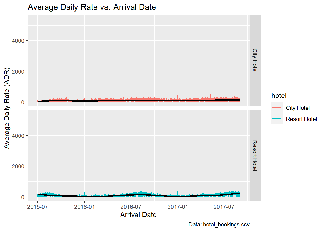
# create a time series graph of adr vs. arrival_date in a facet grid with a least-squares fitted line and labels
ggplot(hotel, aes(`arrival_date`, `adr`, color = `hotel`)) +
  geom_line() +
  facet_grid(rows = vars(`hotel`)) +
  geom_smooth(color = "black") +
  labs(x = "Arrival Date",
       y = "Average Daily Rate (ADR)",
       title = "Average Daily Rate vs. Arrival Date",
       caption = "Data: hotel_bookings.csv"
  )
# zoom in on the time series graphs within the facet grid
ggplot(hotel, aes(`arrival_date`, `adr`, color = `hotel`)) +
  geom_line() +
  facet_grid(rows = vars(`hotel`)) +
  geom_smooth(color = "black") +
  labs(x = "Arrival Date",
       y = "Average Daily Rate (ADR)",
       title = "Average Daily Rate vs. Arrival Date",
       caption = "Data: hotel_bookings.csv"
  ) +
  coord_cartesian(ylim = c(0,600))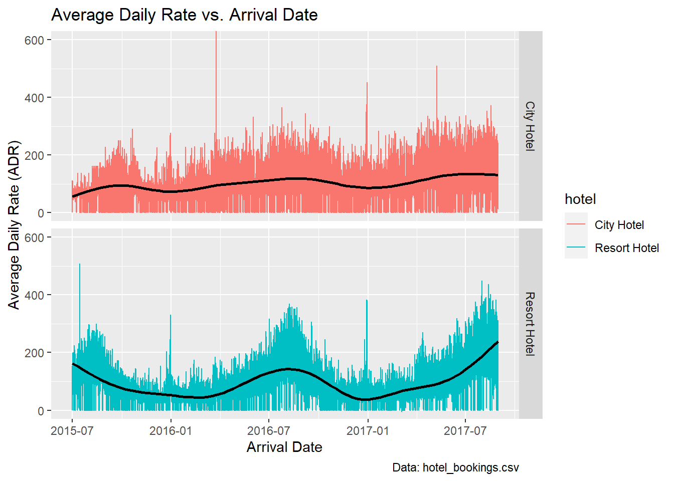
# create a bar graph based on number of bookings vs. deposit type faceted by is_repeated_guest
ggplot(hotel, aes(`deposit_type`, fill = `hotel`)) +
  geom_bar() +
  facet_grid(cols = vars(`is_repeated_guest`)) +
  labs(x = "Deposit Type",
       y = "Number of Bookings",
       title = "Number of Bookings vs. Deposit Type",
       caption = "Data: hotel_bookings.csv",
       subtitle = "Is the booking a repeated guest? \n0 = No \n1 = Yes"
  ) +
  guides(x = guide_axis(n.dodge = 2))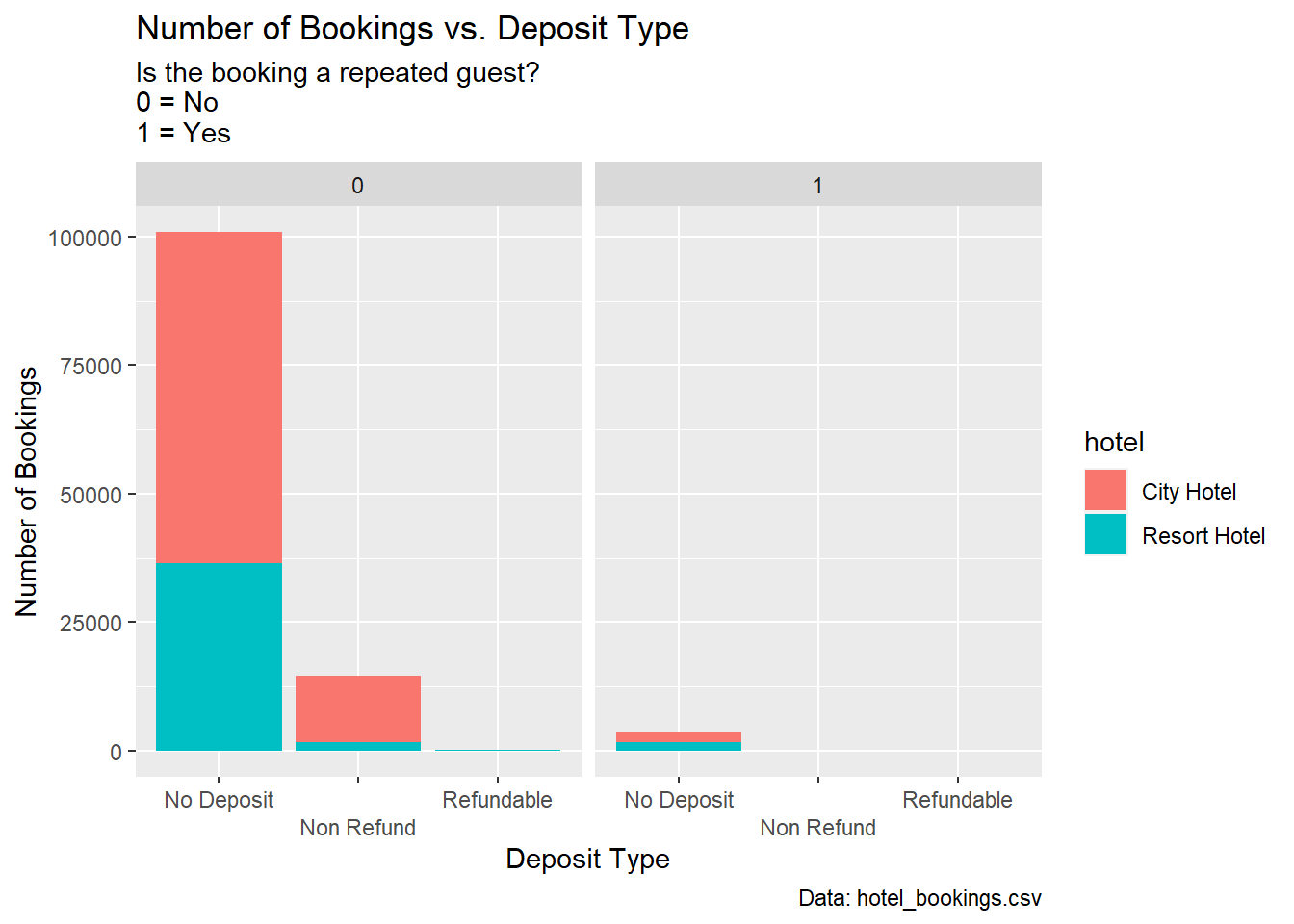
I used the same graphs as I did in Challenge 6 but I added faceting to make each hotel’s data stand out more. For the time series graphs, with the outlier in the city hotel graph, it is difficult to tell how the average daily rate (ADR) varies over time, even with the least-squares fitted line. I decided to use zooming to get a closer look at the area below $600 ADR. It seems like the resort hotel ADR varies more over the span of two years compared to the city hotel ADR. There are also more peaks in ADR over the summer months for the resort hotel. In contrast, the city hotel ADR remains steady or slowly increasing over the years.
For the bar graphs, I added the is_repeated_guest variable to determine whether there is a difference between the deposit type of a first-time guest or regular guest. For first-time guests, there are more bookings without deposits compared to regular guests, with the city hotel having a larger quantity than the resort hotel. This is also reflected with non-refundable deposits. However, there are more refundable deposits for first-time guests than regular guests, especially with the resort hotel. Overall, since there is a larger amount of first-time guests versus repeated guests, we can’t be absolutely certain that there is a difference in deposit type for different types of guests, but the graphs illustrate first-time guests are about as likely to not have to pay a deposit as repeated guests, so there is no special treatment or benefits for being a regular guest.