Code
library(tidyverse)
library(readxl)
library(ggplot2)
library(treemap)

knitr::opts_chunk$set(echo = TRUE)library(tidyverse)
library(readxl)
library(ggplot2)
library(treemap)
knitr::opts_chunk$set(echo = TRUE)Since Homework 3 is a continuation of Homework 2, the sections Read in Data through Potential Research Questions will be the same as Homework 2.
# read in the Current USD sheet of the Milex dataset, skipping the first 6 rows and renaming the columns
milex <- read_excel("_data/SIPRI-Milex-data-1949-2021.xlsx", sheet = "Current USD", skip = 6, col_names = c("Country", "Notes", 1949:2021))
# view milex data
milex
# A tibble: 191 × 75
Country Notes `1949` `1950` `1951` `1952` `1953` `1954` `1955` `1956` `1957`
<chr> <chr> <chr> <chr> <chr> <chr> <chr> <chr> <chr> <chr> <chr>
1 Africa <NA> <NA> <NA> <NA> <NA> <NA> <NA> <NA> <NA> <NA>
2 North A… <NA> <NA> <NA> <NA> <NA> <NA> <NA> <NA> <NA> <NA>
3 Algeria §4 xxx xxx xxx xxx xxx xxx xxx xxx xxx
4 Libya द16 xxx xxx ... ... ... ... ... ... ...
5 Morocco §17 xxx xxx xxx xxx xxx xxx xxx 23.71… 35.40…
6 Tunisia <NA> xxx xxx xxx xxx xxx xxx xxx 3.714… 6.411…
7 sub-Sah… <NA> <NA> <NA> <NA> <NA> <NA> <NA> <NA> <NA> <NA>
8 Angola §‖1 xxx xxx xxx xxx xxx xxx xxx xxx xxx
9 Benin § xxx xxx xxx xxx xxx xxx xxx xxx xxx
10 Botswana <NA> xxx xxx xxx xxx xxx xxx xxx xxx xxx
# … with 181 more rows, and 64 more variables: `1958` <chr>, `1959` <chr>,
# `1960` <chr>, `1961` <chr>, `1962` <chr>, `1963` <chr>, `1964` <chr>,
# `1965` <chr>, `1966` <chr>, `1967` <chr>, `1968` <chr>, `1969` <chr>,
# `1970` <chr>, `1971` <chr>, `1972` <chr>, `1973` <chr>, `1974` <chr>,
# `1975` <chr>, `1976` <chr>, `1977` <chr>, `1978` <chr>, `1979` <chr>,
# `1980` <chr>, `1981` <chr>, `1982` <chr>, `1983` <chr>, `1984` <chr>,
# `1985` <chr>, `1986` <chr>, `1987` <chr>, `1988` <chr>, `1989` <chr>, …milex_clean <- milex %>%
# remove Notes column
select(!contains("Notes")) %>%
# create a column with region names
mutate(Region = case_when(
str_ends(Country, "Africa") ~ "Africa",
str_detect(Country, "America") ~ "Americas",
str_detect(Country, "Asia & Oceania") ~ "Asia & Oceania",
str_ends(Country, "Europe") ~ "Europe",
str_ends(Country, "East") ~ "Middle East",
TRUE ~ NA_character_
)) %>%
# replace NAs in Region column
fill(Region, .direction = "down") %>%
# create a column with sub region names
mutate(Sub_Region = case_when(
str_detect(Country, "North Africa") ~ "North Africa",
str_detect(Country, "sub-Saharan Africa") ~ "sub-Saharan Africa",
str_detect(Country, "Central America and the Caribbean") ~ "Central America and the Caribbean",
str_detect(Country, "North America") ~ "North America",
str_detect(Country, "South America") ~ "South America",
str_detect(Country, "Oceania") ~ "Oceania",
str_detect(Country, "South Asia") ~ "South Asia",
str_detect(Country, "East Asia") ~ "East Asia",
str_detect(Country, "South East Asia") ~ "South East Asia",
str_detect(Country, "Central Asia") ~ "Central Asia",
str_detect(Country, "Central Europe") ~ "Central Europe",
str_detect(Country, "Eastern Europe") ~ "Eastern Europe",
str_detect(Country, "Western Europe") ~ "Western Europe",
str_ends(Country, "East") ~ "Middle East",
TRUE ~ NA_character_
)) %>%
# replace NAs in Sub Region column
fill(Sub_Region, .direction = "down") %>%
# remove rows with region and sub-region names
slice(-c(1:2, 7, 55:56, 70, 73, 85:86, 91, 98, 105, 117, 123:124, 145, 154, 175)) %>%
# replace "xxx" and "..." with NAs
na_if("xxx") %>%
na_if("...") %>%
# combine Region and Sub Region into one column
unite(Region:Sub_Region, col = "Region & Sub Region", sep = "/" ) %>%
# combine year columns into one column
pivot_longer('1949':'2021', names_to = "Year", values_to = "Military Expenditure in Millions of US$")
# view cleaned dataset
milex_clean# A tibble: 12,629 × 4
Country `Region & Sub Region` Year `Military Expenditure in Millions of US$`
<chr> <chr> <chr> <chr>
1 Algeria Africa/North Africa 1949 <NA>
2 Algeria Africa/North Africa 1950 <NA>
3 Algeria Africa/North Africa 1951 <NA>
4 Algeria Africa/North Africa 1952 <NA>
5 Algeria Africa/North Africa 1953 <NA>
6 Algeria Africa/North Africa 1954 <NA>
7 Algeria Africa/North Africa 1955 <NA>
8 Algeria Africa/North Africa 1956 <NA>
9 Algeria Africa/North Africa 1957 <NA>
10 Algeria Africa/North Africa 1958 <NA>
# … with 12,619 more rows# number of distinct countries
n_distinct(milex_clean$Country)[1] 173# list distinct countries
distinct(milex_clean[,1])# A tibble: 173 × 1
Country
<chr>
1 Algeria
2 Libya
3 Morocco
4 Tunisia
5 Angola
6 Benin
7 Botswana
8 Burkina Faso
9 Burundi
10 Cameroon
# … with 163 more rows# list distinct region and sub-region combinations
distinct(milex_clean[,2])# A tibble: 13 × 1
`Region & Sub Region`
<chr>
1 Africa/North Africa
2 Africa/sub-Saharan Africa
3 Americas/Central America and the Caribbean
4 Americas/North America
5 Americas/South America
6 Asia & Oceania/Oceania
7 Asia & Oceania/South Asia
8 Asia & Oceania/East Asia
9 Asia & Oceania/Central Asia
10 Europe/Central Europe
11 Europe/Eastern Europe
12 Europe/Western Europe
13 Middle East/Middle East # number of years
n_distinct(milex_clean$Year)[1] 73# range of years
range(milex_clean$Year)[1] "1949" "2021"The Current USD data from the SIPRI Milex dataset details the military expenditures in millions of US dollars for 173 countries for the period 1949-2021. There are 191 observations (173 actual observations) and 75 variables (Country, Notes, and Years 1949 through 2021). Observations (countries) were grouped by region and sub-region. There are 5 regions (Africa, Americas, Asia & Oceania, Europe, and Middle East) and 14 sub-regions (North Africa, Sub-Saharan Africa, Central America and the Caribbean, North America, South America, Oceania, South Asia, East Asia, South East Asia, Central Asia, Central Europe, Eastern Europe, Western Europe, and Middle East). Some of the data is missing for several countries in various years due to the data not being available or the country did not exist or was not independent at the time the data was collected, so those values are replaced with NAs.
After cleaning the data, the new dataset has 12,629 observations and 4 variables (Country, Region & Sub Region, Year, Military Expenditure in Millions of US$). The regions and sub-regions were extracted from the Country column and combined together into one column to illustrate the various combinations of region and sub-region. The years were also condensed into one column.
Since this data was taken over a large period of time, I can research whether using time series methods would be appropriate to visualize and analyze the trends in the data.
1. What trends are present in the data (e.g. are there certain patterns of military spending over the years)?
2. What are the top spending countries for each year?
3. What is the predicted amount of military expenditures in dollars for year 2022 for each country?
I decided to calculate the average military expenditures (Military Expenditure in Millions of US$) each year (Year) with missing values removed (missing values were removed in all further analyses in order to properly compute these statistics). It appears that the mean military expenditure amount in US dollars steadily increases over time, which makes sense as more warfare and increased tensions between foreign nations began to arise over time. The average military expenditure in US dollars across the entire dataset is 0.6591971. This is about the same as the average in the late 1970s and early 1980s. The standard deviation of military expenditures in millions of US dollars is 0.473998, meaning this data varies about 0.473998 million US dollars from the mean, so given that the mean is 0.6591971 million US dollars, the military expenditure amounts vary quite greatly.
Since there are 13 Region & Sub Region categories, I want to look at the number of times each region and sub region combination is represented in the data. Africa/sub-Saharan Africa is represented the most at 3,431 times with Europe/Central Europe and Europe/Western Europe following at 1,460 times each. This seems correct as there are many sub-Saharan African countries compared to European countries and others. However, I did not specify to remove missing values, so this count may not be entirely accurate as not every country had a military expenditure amount for each year.
Lastly, I computed the average military expenditures in US dollars by country. The range is from 0.05479452 million US dollars to 1 million US dollars, so the USSR has the smallest average while 17 countries (including the United States of America) have the largest average. This is a bit strange since there were a lot of tensions, especially during the Cold War, between the USSR and the USA, but the reason why the USSR has the smallest average military expenditures in US dollars may be because the USSR broke up in the 1990s and most of the larger military expenditures occurred after the disbandment of the USSR.
# calculate the average military expenditures by year
avg_exp <- milex_clean %>%
  group_by(Year) %>%
  summarize(avg_expenditure = mean(!is.na(`Military Expenditure in Millions of US$`)))
# view avg_exp
avg_exp
# A tibble: 73 × 2
Year avg_expenditure
<chr> <dbl>
1 1949 0.0983
2 1950 0.127
3 1951 0.162
4 1952 0.173
5 1953 0.202
6 1954 0.185
7 1955 0.208
8 1956 0.254
9 1957 0.306
10 1958 0.347
# … with 63 more rows# calculate the average military expenditure in millions of US$ across all years
mean(!is.na(milex_clean$`Military Expenditure in Millions of US$`))[1] 0.6591971# compute the standard deviation of military expenditures in millions of US$
sd(!is.na(milex_clean$`Military Expenditure in Millions of US$`))[1] 0.473998# count region & sub region combinations
region_subregion <- milex_clean %>%
group_by(`Region & Sub Region`) %>%
summarize(n = n())
# view region_subregion
region_subregion# A tibble: 13 × 2
`Region & Sub Region` n
<chr> <int>
1 Africa/North Africa 292
2 Africa/sub-Saharan Africa 3431
3 Americas/Central America and the Caribbean 949
4 Americas/North America 146
5 Americas/South America 803
6 Asia & Oceania/Central Asia 365
7 Asia & Oceania/East Asia 1241
8 Asia & Oceania/Oceania 292
9 Asia & Oceania/South Asia 438
10 Europe/Central Europe 1460
11 Europe/Eastern Europe 584
12 Europe/Western Europe 1460
13 Middle East/Middle East 1168# compute average military expenditures by country
country_exp <- milex_clean %>%
group_by(Country) %>%
summarize(avg_expenditure = mean(!is.na(`Military Expenditure in Millions of US$`)))
# view country_exp
country_exp# A tibble: 173 × 2
Country avg_expenditure
<chr> <dbl>
1 Afghanistan 0.329
2 Albania 0.644
3 Algeria 0.808
4 Angola 0.603
5 Argentina 1
6 Armenia 0.397
7 Australia 1
8 Austria 0.890
9 Azerbaijan 0.411
10 Bahrain 0.699
# … with 163 more rows# find the range of the average military expenditures in millions of US$ out of all countries
range(country_exp$avg_expenditure)[1] 0.05479452 1.00000000# find the country with the smallest average military expenditure in US$
slice_min(country_exp, avg_expenditure)# A tibble: 1 × 2
Country avg_expenditure
<chr> <dbl>
1 USSR 0.0548# find the countries with the largest average military expenditure in US$
slice_max(country_exp, avg_expenditure)# A tibble: 17 × 2
Country avg_expenditure
<chr> <dbl>
1 Argentina 1
2 Australia 1
3 Belgium 1
4 Costa Rica 1
5 Denmark 1
6 France 1
7 Greece 1
8 Italy 1
9 Luxembourg 1
10 Mexico 1
11 Netherlands 1
12 Norway 1
13 Peru 1
14 Portugal 1
15 Spain 1
16 Turkey 1
17 United States of America 1# find the top 5 spending countries for each year
top_country_exp <- milex_clean %>%
group_by(Year) %>%
arrange(desc(`Military Expenditure in Millions of US$`)) %>%
slice_head(n = 5)
# view top_country_exp
top_country_exp# A tibble: 365 × 4
# Groups: Year [73]
Country `Region & Sub Region` Year Military Expendit…¹
<chr> <chr> <chr> <chr>
1 Denmark Europe/Western Europe 1949 69.297401347449465
2 Norway Europe/Western Europe 1949 67.17745742401685
3 Portugal Europe/Western Europe 1949 54.441128511214352
4 Italy Europe/Western Europe 1949 467.23430058061933
5 Mexico Americas/Central America and the Caribbean 1949 34.797687861271676
6 Chile Americas/South America 1950 87.502552157771277
7 Portugal Europe/Western Europe 1950 52.732141362862961
8 Denmark Europe/Western Europe 1950 51.975202471645282
9 Italy Europe/Western Europe 1950 501.26509684299299
10 Norway Europe/Western Europe 1950 49.979980008007999
# … with 355 more rows, and abbreviated variable name
# ¹`Military Expenditure in Millions of US$`# filter the top 5 spending countries from 1949 to 1953
first_5_yrs <- filter(top_country_exp, Year <= 1953)
# view first 5 years data frame
first_5_yrs# A tibble: 25 × 4
# Groups: Year [5]
Country `Region & Sub Region` Year Military Expendit…¹
<chr> <chr> <chr> <chr>
1 Denmark Europe/Western Europe 1949 69.297401347449465
2 Norway Europe/Western Europe 1949 67.17745742401685
3 Portugal Europe/Western Europe 1949 54.441128511214352
4 Italy Europe/Western Europe 1949 467.23430058061933
5 Mexico Americas/Central America and the Caribbean 1949 34.797687861271676
6 Chile Americas/South America 1950 87.502552157771277
7 Portugal Europe/Western Europe 1950 52.732141362862961
8 Denmark Europe/Western Europe 1950 51.975202471645282
9 Italy Europe/Western Europe 1950 501.26509684299299
10 Norway Europe/Western Europe 1950 49.979980008007999
# … with 15 more rows, and abbreviated variable name
# ¹`Military Expenditure in Millions of US$`# filter the top 5 spending countries from 2017 to 2021
last_5_yrs <- filter(top_country_exp, Year >= 2017)
# view last 5 years data frame
last_5_yrs# A tibble: 25 × 4
# Groups: Year [5]
Country `Region & Sub Region` Year Military Expenditure in Millio…¹
<chr> <chr> <chr> <chr>
1 Poland Europe/Central Europe 2017 9870.6806282722519
2 Korea, North Asia & Oceania/East Asia 2017 961.48148148148152
3 Netherlands Europe/Western Europe 2017 9580.6854982163022
4 Croatia Europe/Central Europe 2017 920.83705291818819
5 Cape Verde Africa/sub-Saharan Africa 2017 9.3543841662816174
6 Croatia Europe/Central Europe 2018 966.35871679888726
7 Bulgaria Europe/Central Europe 2018 961.29727459449623
8 Mongolia Asia & Oceania/East Asia 2018 96.067489859811118
9 Algeria Africa/North Africa 2018 9583.7242883703002
10 Eswatini Africa/sub-Saharan Africa 2018 95.863380323095569
# … with 15 more rows, and abbreviated variable name
# ¹`Military Expenditure in Millions of US$`To visualize trends of military expenditures over time, I created a time series plot of avg_expenditure vs. year from the avg_exp data frame. To reiterate, missing values are not included in order to proceed with the analysis. As we can see from the plot, there is a clear increasing trend of military expenditures over time, with the data stabilizing around the late 2010s. As previously mentioned, there was quite a bit of warfare and rising tensions in the twentieth century but the reasoning behind the increasing trend leveling off later on may be due to some countries making an effort to decrease or cut military spending in order to not raise their national debt or the global COVID-19 pandemic taking place beginning in late 2019 and early 2020.
The second visualization is a tree map depicting the region and sub region counts by the sizes of the rectangles. Africa/sub-Saharan Africa is the largest rectangle which coincides with my observation in the previous section. Although Europe/Central Europe and Europe/Western Europe have the same count, their rectangles look different as Europe/Central Europe is longer and Europe/Western Europe looks wider. It would be easier to tell if the counts were listed under the labels but I did not find out how to do this.
These third and fourth visualizations illustrate the top five spending countries for the first five years and last five years respectively. The military expenditures in US millions of dollars have a wider range in the first five years of data versus the last five years of data, with the first five years ranging from 34 million US dollars to 986 million US dollars and the last five years ranging from 85 to 9,978 million US dollars. What I find interesting are the countries that repeatedly rank in the top five: for example, Denmark was in the top five for 1949 to 1952 while Algeria was in the top five for 2018, 2020, and 2021. I’m not up-to-date on world relations and current events, but for a country to be in the top five for military expenditures, most likely the military makes up a large portion of the country’s budget and is therefore an important asset for them to maintain.
# create a time series plot of avg_expenditure vs. year with avg_exp data
ggplot(avg_exp, aes(Year, avg_expenditure)) +
  geom_point() +
  guides(x = guide_axis(n.dodge = 5)) +
  labs(x = "Year",
       y = "Average Expenditure in Millions (US$)",
       title = "Time Series of Average Expenditure in Millions (US$) vs. Year",
       subtitle = "Missing values are not included",
       caption = "Data: SIPRI-Milex-data-1949-2021.xlsx")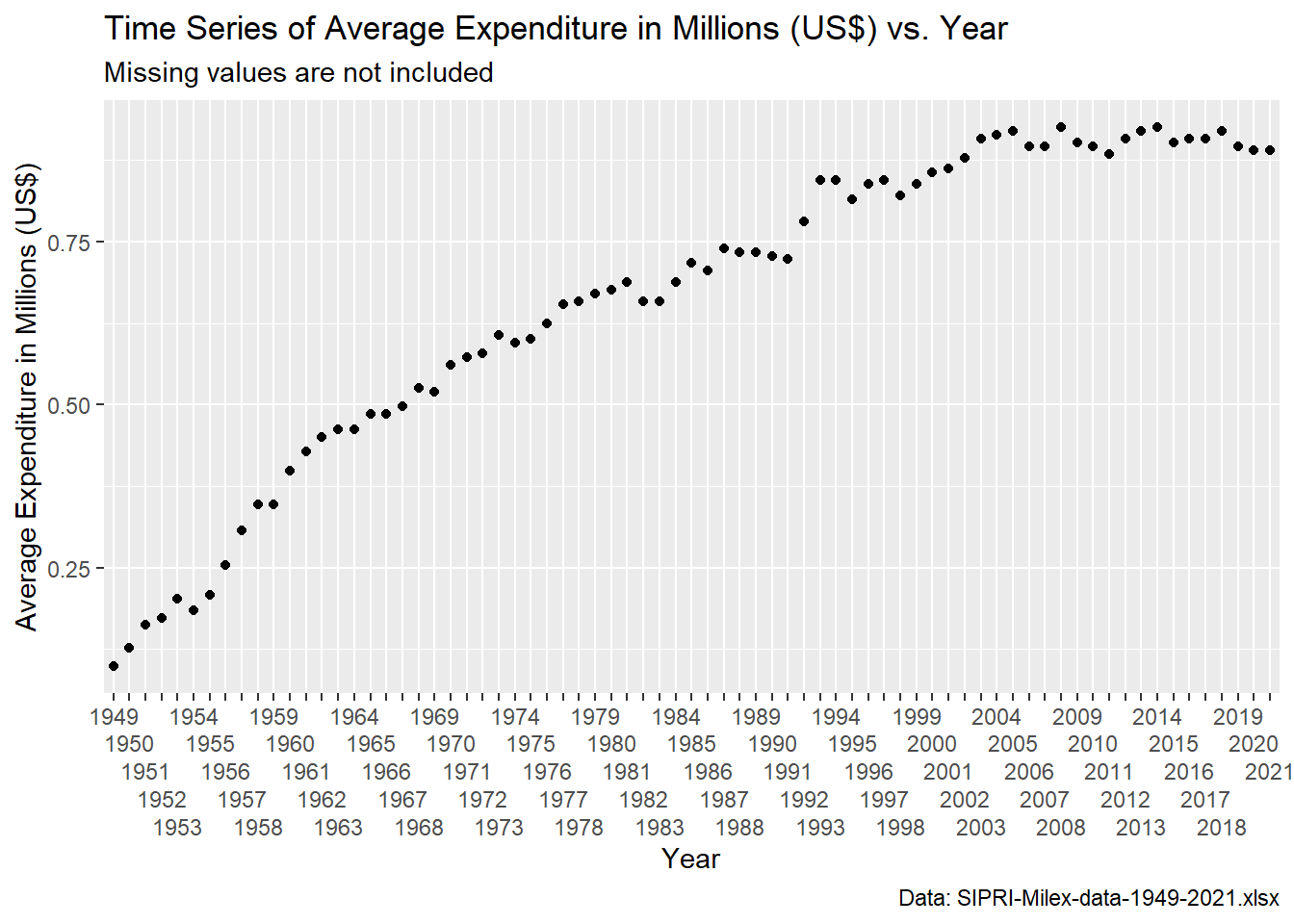
# create a treemap of region and sub region counts
treemap(region_subregion,
            index="Region & Sub Region",
            vSize="n",
            type="index",
            title="Treemap of Region & Sub Region Counts",
            fontsize.title = 12)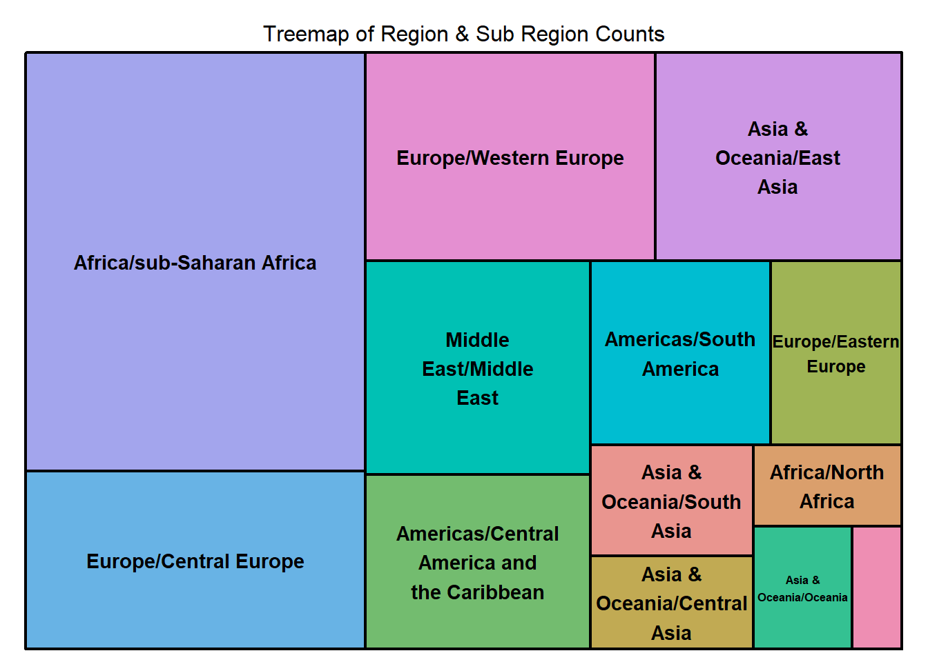
# create a scatterplot of military expenditure in millions of US$ vs. year with top 5 highest spending countries from 1949 to 1953
ggplot(first_5_yrs, aes(Year, `Military Expenditure in Millions of US$`)) +
  geom_point(aes(color = Country)) +
  theme(legend.position = "bottom") +
  labs(title = "Scatterplot of Top 5 Highest Spending Countries from 1949 to 1953",
       caption = "Data: SIPRI-Milex-data-1949-2021.xlsx")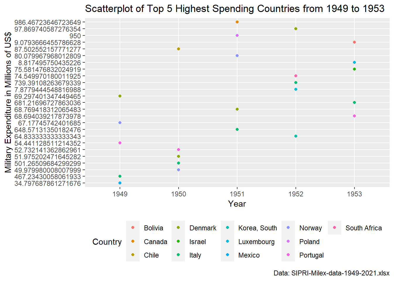
# create a scatterplot of military expenditure in millions of US$ vs. year with top 5 highest spending countries from 2017 to 2021
ggplot(last_5_yrs, aes(Year, `Military Expenditure in Millions of US$`)) +
  geom_point(aes(color = Country)) +
  theme(legend.position = "bottom") +
  labs(title = "Scatterplot of Top 5 Highest Spending Countries from 2017 to 2021",
       caption = "Data: SIPRI-Milex-data-1949-2021.xlsx")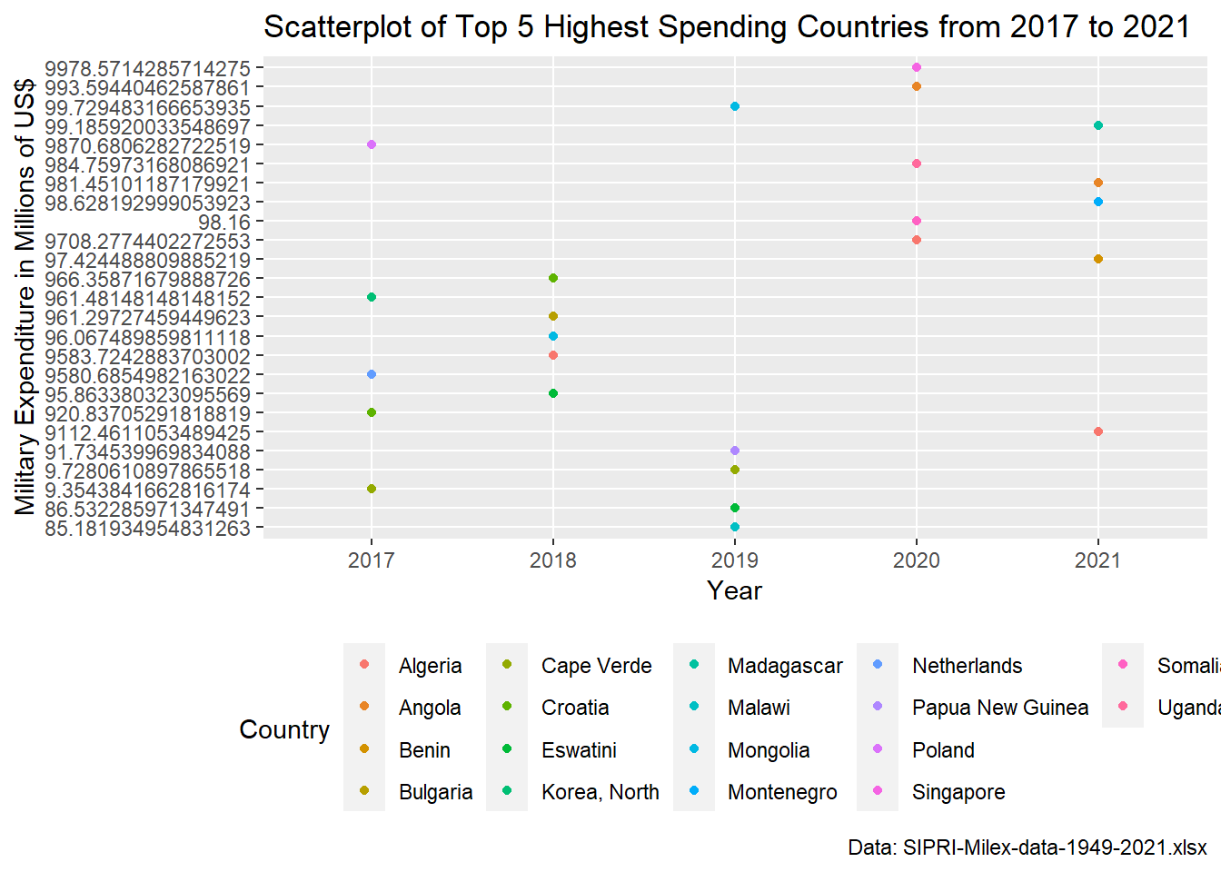
The biggest limitation to my visualizations is in relation to my third research question: What is the predicted amount of military expenditures in dollars for year 2022 for each country? I unfortunately ran out of time and space for this assignment to go in depth into this question but I would assume based on my math background, this would require some forecasting techniques. I would like to dive into more prediction-related analysis to answer this question, but this is outside the scope of this class, so I will have to come back to it later on after a refresher on forecasting methods.
As for the top spending countries of each year, it was very difficult to visualize the top five spending countries from 1949 to 2021 in one plot (or even faceted plots) which is why I had to limit to illustrating only the first five years (1949 to 1953) and the last five years (2017 to 2021). It would be better for comparison to display all the years in one chart but that was not possible. However, from what I was able to do, I could draw a good conclusion as to what the data was portraying. For the final project, I think it would be beneficial to look more into faceting and other techniques regarding fitting all data points in one plot. In addition, I’ll also conduct further research on how to improve my titles and labels on my graphs as they can be better than they are now.