Challenge 3 Instructions

Code

library(tidyverse)

knitr::opts_chunk$set(echo = TRUE, warning=FALSE, message=FALSE)

Challenge Overview

Today’s challenge is to:

1. read in a data set, and describe the data set using both words and any supporting information (e.g., tables, etc)
2. identify what needs to be done to tidy the current data
3. anticipate the shape of pivoted data
4. pivot the data into tidy format using pivot_longer

Read in data

Read in one (or more) of the following datasets, using the correct R package and command.

• animal_weights.csv ⭐
• eggs_tidy.csv ⭐⭐ or organiceggpoultry.xls ⭐⭐⭐
• australian_marriage*.xls ⭐⭐⭐
• USA Households*.xlsx ⭐⭐⭐⭐
• sce_labor_chart_data_public.xlsx 🌟🌟🌟🌟🌟

Code

library(readr)
 eggs<- read_csv("_data/eggs_tidy.csv")
eggs

# A tibble: 120 × 6
   month      year large_half_dozen large_dozen extra_large_half_dozen extra_l…¹
   <chr>     <dbl>            <dbl>       <dbl>                  <dbl>     <dbl>
 1 January    2004             126         230                    132       230 
 2 February   2004             128.        226.                   134.      230 
 3 March      2004             131         225                    137       230 
 4 April      2004             131         225                    137       234.
 5 May        2004             131         225                    137       236 
 6 June       2004             134.        231.                   137       241 
 7 July       2004             134.        234.                   137       241 
 8 August     2004             134.        234.                   137       241 
 9 September  2004             130.        234.                   136.      241 
10 October    2004             128.        234.                   136.      241 
# … with 110 more rows, and abbreviated variable name ¹​extra_large_dozen

Code

# Data set of large and extra large in one column 

eggs_long<-eggs%>%
  pivot_longer(cols=contains("large"), 
               names_to = "eggType",
               values_to = "avgPrice"
  )

eggs_long<- eggs_long%>%
  mutate(size = case_when(startsWith(eggType, "extra")~"extra_large",startsWith(eggType, "large")~"large"))




#boxplot for large eggs and there weights 
ggplot(eggs_long, aes(x=size, y=avgPrice, col=size)) + geom_boxplot()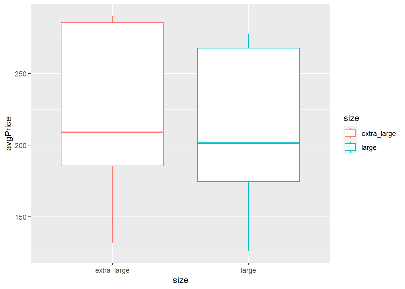

Code

#boxplot + Facet grid for large eggs by year and weight 
ggplot(large, aes(x="", y=weight)) + geom_boxplot()+ facet_grid(large~year)

Error in ggplot(large, aes(x = "", y = weight)): object 'large' not found

Code

#egg count per month 
eggs %>% 
  count(month)

# A tibble: 12 × 2
   month         n
   <chr>     <int>
 1 April        10
 2 August       10
 3 December     10
 4 February     10
 5 January      10
 6 July         10
 7 June         10
 8 March        10
 9 May          10
10 November     10
11 October      10
12 September    10

Code

#egg count per year 
eggs %>%
  count(year)

# A tibble: 10 × 2
    year     n
   <dbl> <int>
 1  2004    12
 2  2005    12
 3  2006    12
 4  2007    12
 5  2008    12
 6  2009    12
 7  2010    12
 8  2011    12
 9  2012    12
10  2013    12

Briefly describe the data

the data contained in the first code is a pivot to tidy the table and to select avg price of the values.

#second code The second code is creating a boxplot diagram for the large eggs and the weights

#the third code Includes a facet grid for all years by egg weights for large eggs

#4th code For count of eggs per month

#5th code Count of eggs per year

Anticipate the End Result

The first step in pivoting the data is to try to come up with a concrete vision of what the end product should look like - that way you will know whether or not your pivoting was successful.

One easy way to do this is to think about the dimensions of your current data (tibble, dataframe, or matrix), and then calculate what the dimensions of the pivoted data should be.

Suppose you have a dataset with \(n\) rows and \(k\) variables. In our example, 3 of the variables are used to identify a case, so you will be pivoting \(k-3\) variables into a longer format where the \(k-3\) variable names will move into the names_to variable and the current values in each of those columns will move into the values_to variable. Therefore, we would expect \(n * (k-3)\) rows in the pivoted dataframe!

Example: find current and future data dimensions

Lets see if this works with a simple example.

Code

df

function (x, df1, df2, ncp, log = FALSE) 
{
    if (missing(ncp)) 
        .Call(C_df, x, df1, df2, log)
    else .Call(C_dnf, x, df1, df2, ncp, log)
}
<bytecode: 0x000001bff0754d30>
<environment: namespace:stats>

Code

df<-tibble(eggs = rep(c("large", "extra_large", "year"),2),
           year = rep(c(2004,2013), 3), 
           trade = rep(c(),2),
           outgoing = rnorm(6, mean=1000, sd=500),
           incoming = rlogis(6, location=1000, 
                             scale = 400))
df

# A tibble: 6 × 4
  eggs         year outgoing incoming
  <chr>       <dbl>    <dbl>    <dbl>
1 large        2004    1651.   1364. 
2 extra_large  2013    1724.   -340. 
3 year         2004     942.   1489. 
4 large        2013     803.    -95.8
5 extra_large  2004    1144.    214. 
6 year         2013    1299.    638. 

Code

#existing rows/cases
nrow(df)

[1] 6

Code

#existing columns/cases
ncol(df)

[1] 4

Code

#expected rows/cases
nrow(df) * (ncol(df)-3)

[1] 6

Code

# expected columns 
3 + 2

[1] 5

Or simple example has \(n = 6\) rows and \(k - 3 = 2\) variables being pivoted, so we expect a new dataframe to have \(n * 2 = 12\) rows x \(3 + 2 = 5\) columns.

Challenge: Describe the final dimensions

Document your work here.

Any additional comments?

Pivot the Data

Now we will pivot the data, and compare our pivoted data dimensions to the dimensions calculated above as a “sanity” check.

Example

Code

df<-pivot_longer(df, col = c(outgoing, incoming),
                 names_to="trade_direction",
                 values_to = "trade_value")
df

# A tibble: 12 × 4
   eggs         year trade_direction trade_value
   <chr>       <dbl> <chr>                 <dbl>
 1 large        2004 outgoing             1651. 
 2 large        2004 incoming             1364. 
 3 extra_large  2013 outgoing             1724. 
 4 extra_large  2013 incoming             -340. 
 5 year         2004 outgoing              942. 
 6 year         2004 incoming             1489. 
 7 large        2013 outgoing              803. 
 8 large        2013 incoming              -95.8
 9 extra_large  2004 outgoing             1144. 
10 extra_large  2004 incoming              214. 
11 year         2013 outgoing             1299. 
12 year         2013 incoming              638. 

Yes, once it is pivoted long, our resulting data are \(12x5\) - exactly what we expected!

Challenge: Pivot the Chosen Data

Document your work here. What will a new “case” be once you have pivoted the data? How does it meet requirements for tidy data? Any additional comments?