Homework 1

Code

library(tidyverse)
library(readxl)
library(ggplot2)
options(scipen=999)
knitr::opts_chunk$set(echo = TRUE)

old<-options(pillar.sigfig = 2)

With only skipping the first line here is what wild_bird_data.xlsx looks like

Code

birdsData <- read_excel("_data/wild_bird_data.xlsx",skip=1)
birdsData%>%
  head()%>%
  arrange(`Wet body weight [g]`)

# A tibble: 6 × 2
  `Wet body weight [g]` `Population size`
                  <dbl>             <dbl>
1                   5.5           532194.
2                   7.4           389806.
3                   7.8          3165107.
4                   8.6          2592997.
5                   9.1           604766.
6                  11.           3524193.

While this data source is lacking the names of each bird, it appears the wet body weight in grams was collected for a variety of birds(146). This weight is then tied to an estimated population size, I say estimated because the numbers are not integers.

Wet body weight[g] reflects the weight of a particular bird while alive as well as that birds (est?) population size.

Code

count(birdsData)

# A tibble: 1 × 1
      n
  <int>
1   146

Body weight stats

Smallest bird:

Code

smallestBird<-birdsData%>%
  slice(1)

smallestBird

# A tibble: 1 × 2
  `Wet body weight [g]` `Population size`
                  <dbl>             <dbl>
1                   5.5           532194.

Largest bird:

Code

birdsData%>%
  tail(n=1)

# A tibble: 1 × 2
  `Wet body weight [g]` `Population size`
                  <dbl>             <dbl>
1                 2054.            20661.

To give some perspective:

Robin average weight: 70g.

Pelican average weight: 11,000g

Average

Code

birdsData%>%
  summarise('average weight'=mean(`Wet body weight [g]`))

# A tibble: 1 × 1
  `average weight`
             <dbl>
1             364.

population size vs body weight plot

Here I wanted to show how body weight correlates with population size. The raw chart had some outliers which led me to focus in on birds with a body weight of less than 2.5kgs

raw graph

Code

graph<-
  birdsData%>%
  ggplot(aes(`Wet body weight [g]`,`Population size`)) + geom_point() + geom_smooth(method="lm")

graph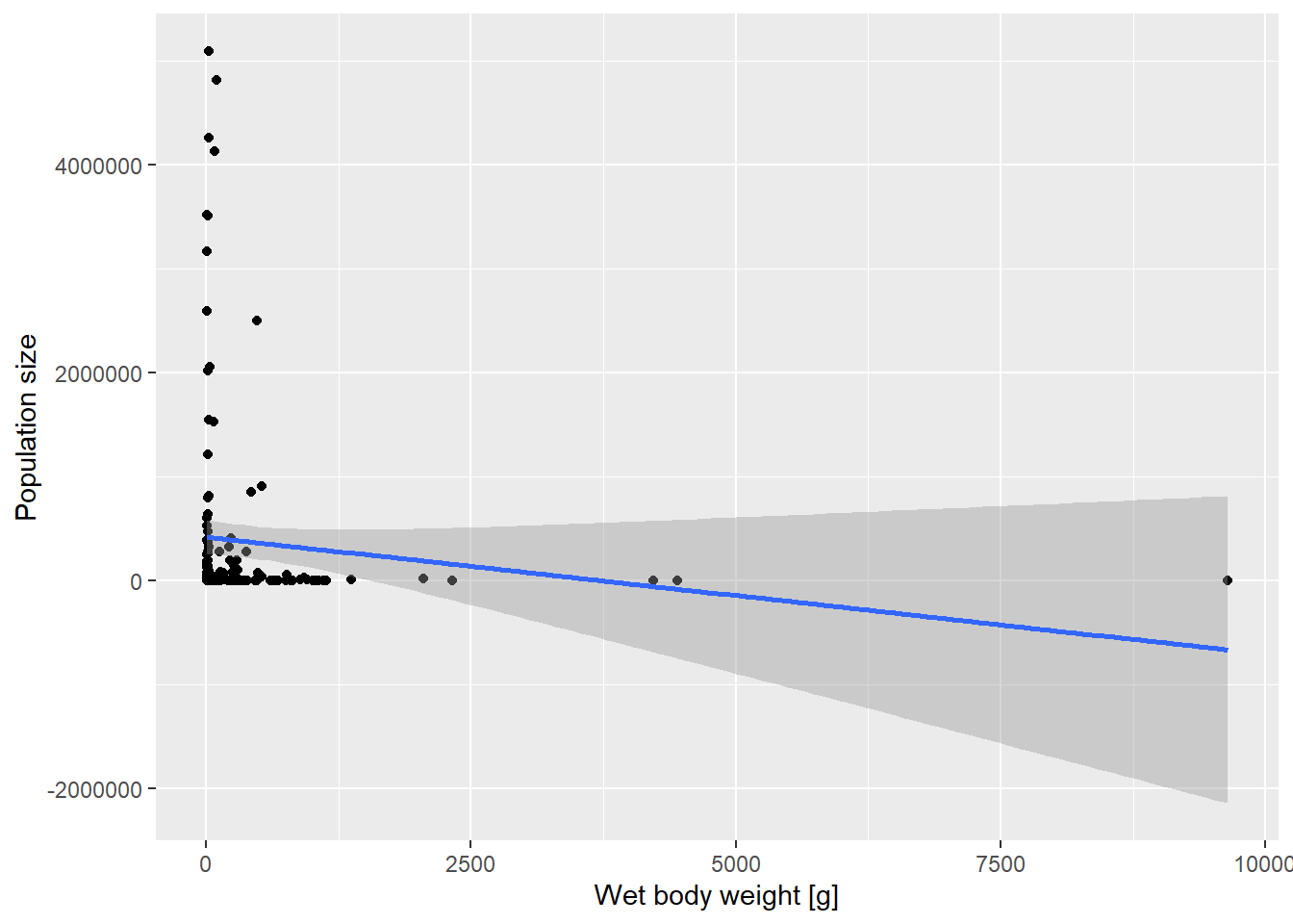

With constraints

We see once we focus in on smaller birds, weight< 500g, a bit more of a clear trend in pop size vs weight

Code

graph + xlim(c(0, 500))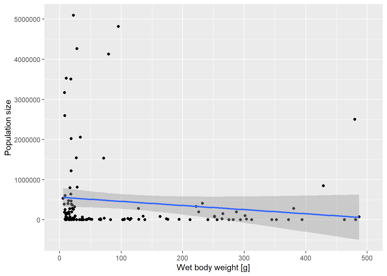 

Conclusions

This data could be used to draw conclusions about the populations of birds based on their wet body mass.