Challenge 2

challenge_2

birds

Author

Julian Castoro

Published

August 16, 2022

Code

library(tidyverse)
library(dplyr)
library(readxl)
library(ggplot2)

options(scipen=999)


knitr::opts_chunk$set(echo = TRUE, warning=FALSE, message=FALSE)

! Question: How would i find the difference between first and last years Value cols for each category in each region? !

Challenge Overview

Today’s challenge is to

read in a data set, and describe the data using both words and any supporting information (e.g., tables, etc)
provide summary statistics for different interesting groups within the data, and interpret those statistics

Read in the Data

Read in one (or more) of the following data sets, available in the posts/_data folder, using the correct R package and command.

birds.csv ⭐⭐⭐

Code

birdsData <- read_csv("_data/birds.csv")
birdsData

# A tibble: 30,977 × 14
   Domain Cod…¹ Domain Area …² Area  Eleme…³ Element Item …⁴ Item  Year …⁵  Year
   <chr>        <chr>    <dbl> <chr>   <dbl> <chr>     <dbl> <chr>   <dbl> <dbl>
 1 QA           Live …       2 Afgh…    5112 Stocks     1057 Chic…    1961  1961
 2 QA           Live …       2 Afgh…    5112 Stocks     1057 Chic…    1962  1962
 3 QA           Live …       2 Afgh…    5112 Stocks     1057 Chic…    1963  1963
 4 QA           Live …       2 Afgh…    5112 Stocks     1057 Chic…    1964  1964
 5 QA           Live …       2 Afgh…    5112 Stocks     1057 Chic…    1965  1965
 6 QA           Live …       2 Afgh…    5112 Stocks     1057 Chic…    1966  1966
 7 QA           Live …       2 Afgh…    5112 Stocks     1057 Chic…    1967  1967
 8 QA           Live …       2 Afgh…    5112 Stocks     1057 Chic…    1968  1968
 9 QA           Live …       2 Afgh…    5112 Stocks     1057 Chic…    1969  1969
10 QA           Live …       2 Afgh…    5112 Stocks     1057 Chic…    1970  1970
# … with 30,967 more rows, 4 more variables: Unit <chr>, Value <dbl>,
#   Flag <chr>, `Flag Description` <chr>, and abbreviated variable names
#   ¹`Domain Code`, ²`Area Code`, ³`Element Code`, ⁴`Item Code`, ⁵`Year Code`

testing different groupings

Grouping by item and tallying we see the below counts of rows of information on each of the types of birds in this dataset.

Code

by_item <- birdsData %>% group_by(Item)
by_item %>% tally()

# A tibble: 5 × 2
  Item                       n
  <chr>                  <int>
1 Chickens               13074
2 Ducks                   6909
3 Geese and guinea fowls  4136
4 Pigeons, other birds    1165
5 Turkeys                 5693

Summarizing by count shows us the total amount of birds in each category. (NA’s removed)

Code

summarize(by_item, count=sum(Value,na.rm = TRUE))

# A tibble: 5 × 2
  Item                        count
  <chr>                       <dbl>
1 Chickens               2696862583
2 Ducks                   149781301
3 Geese and guinea fowls   41136874
4 Pigeons, other birds      6822856
5 Turkeys                  81850064

Summarizing the Grouping by area and Item gives us the mean number of each item type from 1961-2018 (Where a value exists)

Code

by_area <- birdsData %>% group_by(Area,Item)
by_area

# A tibble: 30,977 × 14
# Groups:   Area, Item [601]
   Domain Cod…¹ Domain Area …² Area  Eleme…³ Element Item …⁴ Item  Year …⁵  Year
   <chr>        <chr>    <dbl> <chr>   <dbl> <chr>     <dbl> <chr>   <dbl> <dbl>
 1 QA           Live …       2 Afgh…    5112 Stocks     1057 Chic…    1961  1961
 2 QA           Live …       2 Afgh…    5112 Stocks     1057 Chic…    1962  1962
 3 QA           Live …       2 Afgh…    5112 Stocks     1057 Chic…    1963  1963
 4 QA           Live …       2 Afgh…    5112 Stocks     1057 Chic…    1964  1964
 5 QA           Live …       2 Afgh…    5112 Stocks     1057 Chic…    1965  1965
 6 QA           Live …       2 Afgh…    5112 Stocks     1057 Chic…    1966  1966
 7 QA           Live …       2 Afgh…    5112 Stocks     1057 Chic…    1967  1967
 8 QA           Live …       2 Afgh…    5112 Stocks     1057 Chic…    1968  1968
 9 QA           Live …       2 Afgh…    5112 Stocks     1057 Chic…    1969  1969
10 QA           Live …       2 Afgh…    5112 Stocks     1057 Chic…    1970  1970
# … with 30,967 more rows, 4 more variables: Unit <chr>, Value <dbl>,
#   Flag <chr>, `Flag Description` <chr>, and abbreviated variable names
#   ¹`Domain Code`, ²`Area Code`, ³`Element Code`, ⁴`Item Code`, ⁵`Year Code`

Code

summarise(by_area, birds = round(mean(Value, na.rm = TRUE)))

# A tibble: 601 × 3
# Groups:   Area [248]
   Area        Item                    birds
   <chr>       <chr>                   <dbl>
 1 Afghanistan Chickens                 8099
 2 Africa      Chickens               936779
 3 Africa      Ducks                   13639
 4 Africa      Geese and guinea fowls  12164
 5 Africa      Pigeons, other birds    11222
 6 Africa      Turkeys                  9004
 7 Albania     Chickens                 4055
 8 Albania     Ducks                     558
 9 Albania     Geese and guinea fowls    396
10 Albania     Turkeys                   750
# … with 591 more rows

Describe the data

Using a combination of words and results of R commands, can you provide a high level description of the data? Describe as efficiently as possible where/how the data was (likely) gathered, indicate the cases and variables (both the interpretation and any details you deem useful to the reader to fully understand your chosen data).

This data appears to be about the amounts of different varieties of bird category by area/region over time. Based on the variety of different collection methods seen below, we can assume this info is a conglomeration from a few sources.

FAO stands for the food and agriculture association

Code

unique(birdsData$`Flag Description`)

[1] "FAO estimate"                                                                
[2] "Official data"                                                               
[3] "FAO data based on imputation methodology"                                    
[4] "Data not available"                                                          
[5] "Unofficial figure"                                                           
[6] "Aggregate, may include official, semi-official, estimated or calculated data"

An interesting area I wanted to filter on was the flag for how the data was collected.

Due to using the “na.rm = true” modifier in my earlier code, we never included any rows where the data was not available however we may want to see only official data.

Below we see a snapshot of the most recent and official data

Code

by_area_year <- birdsData %>% group_by(Area,Year,Item)
by_area_year

# A tibble: 30,977 × 14
# Groups:   Area, Year, Item [30,977]
   Domain Cod…¹ Domain Area …² Area  Eleme…³ Element Item …⁴ Item  Year …⁵  Year
   <chr>        <chr>    <dbl> <chr>   <dbl> <chr>     <dbl> <chr>   <dbl> <dbl>
 1 QA           Live …       2 Afgh…    5112 Stocks     1057 Chic…    1961  1961
 2 QA           Live …       2 Afgh…    5112 Stocks     1057 Chic…    1962  1962
 3 QA           Live …       2 Afgh…    5112 Stocks     1057 Chic…    1963  1963
 4 QA           Live …       2 Afgh…    5112 Stocks     1057 Chic…    1964  1964
 5 QA           Live …       2 Afgh…    5112 Stocks     1057 Chic…    1965  1965
 6 QA           Live …       2 Afgh…    5112 Stocks     1057 Chic…    1966  1966
 7 QA           Live …       2 Afgh…    5112 Stocks     1057 Chic…    1967  1967
 8 QA           Live …       2 Afgh…    5112 Stocks     1057 Chic…    1968  1968
 9 QA           Live …       2 Afgh…    5112 Stocks     1057 Chic…    1969  1969
10 QA           Live …       2 Afgh…    5112 Stocks     1057 Chic…    1970  1970
# … with 30,967 more rows, 4 more variables: Unit <chr>, Value <dbl>,
#   Flag <chr>, `Flag Description` <chr>, and abbreviated variable names
#   ¹`Domain Code`, ²`Area Code`, ³`Element Code`, ⁴`Item Code`, ⁵`Year Code`

Code

by_area_year %>%
filter(`Flag Description` == "Official data",Year == 2018) %>%
  summarise(NumberOfBirds = Value)

# A tibble: 135 × 4
# Groups:   Area, Year [66]
   Area                    Year Item     NumberOfBirds
   <chr>                  <dbl> <chr>            <dbl>
 1 Albania                 2018 Chickens          7272
 2 Albania                 2018 Turkeys            403
 3 Argentina               2018 Chickens        113600
 4 Armenia                 2018 Chickens          4406
 5 Azerbaijan              2018 Chickens         30498
 6 Bangladesh              2018 Chickens        282145
 7 Bangladesh              2018 Ducks            55853
 8 Belgium                 2018 Chickens         32327
 9 Benin                   2018 Chickens         21304
10 Bosnia and Herzegovina  2018 Chickens         16229
# … with 125 more rows

Next I add a calculated field to see how the populations have changed over the years. As a test I will be exploring Belgium.

Code

by_area_year%>%
  filter(Area == "Belgium")%>%
  ggplot(aes(Year,Value)) + geom_line(aes(color=Item)) +geom_point()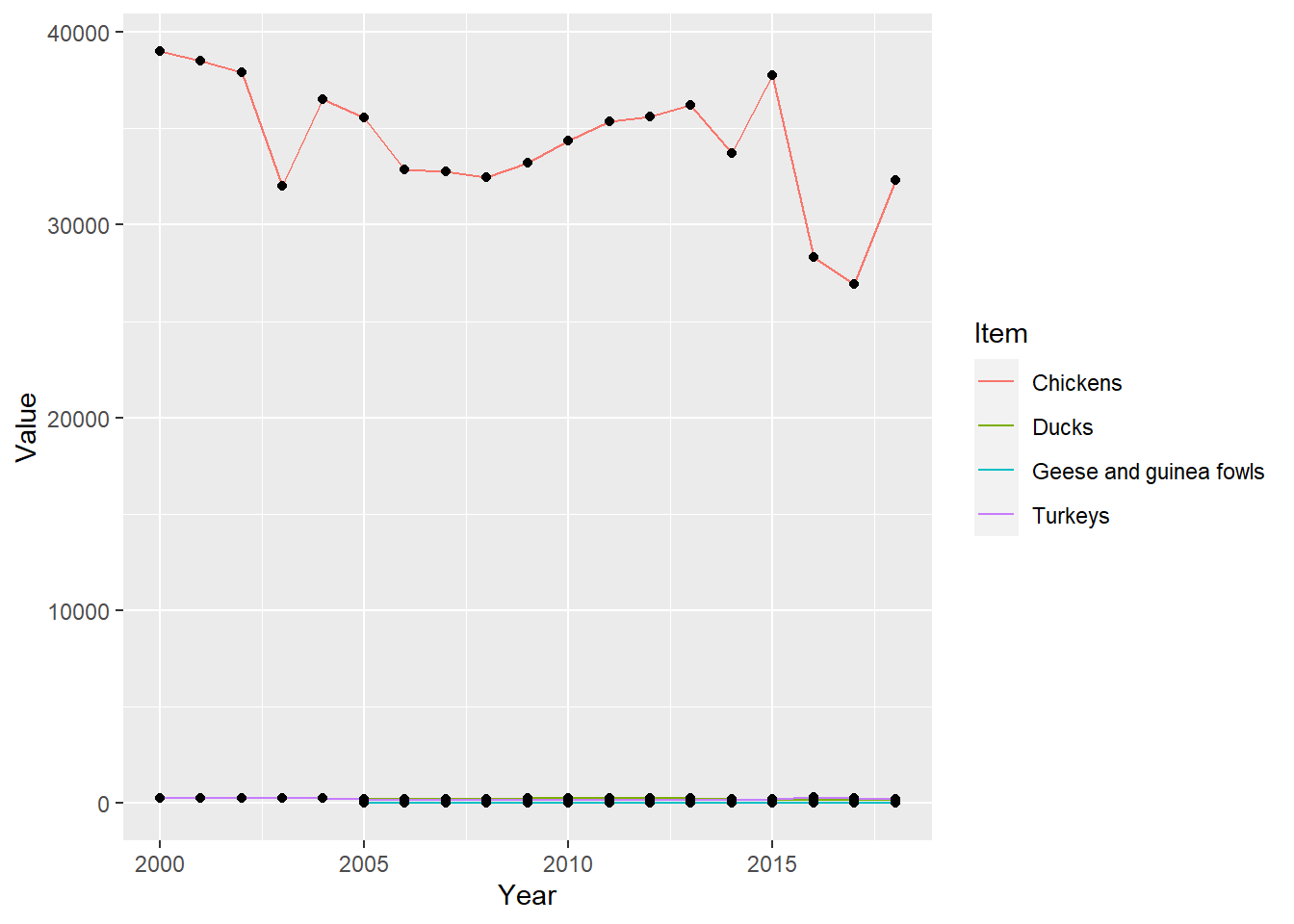

After making this chart I wanted to know what the entire pool of sampled areas chicken populations might have looked like.

Code

Chickens_by_area_year <- birdsData %>% filter(Item == "Chickens", Area != "World")%>%group_by(Area,Year)
Chickens_by_area_year %>%
  ggplot(aes(Year,Value)) + geom_line(aes(color=Area)) +geom_point() + theme(legend.position = "none")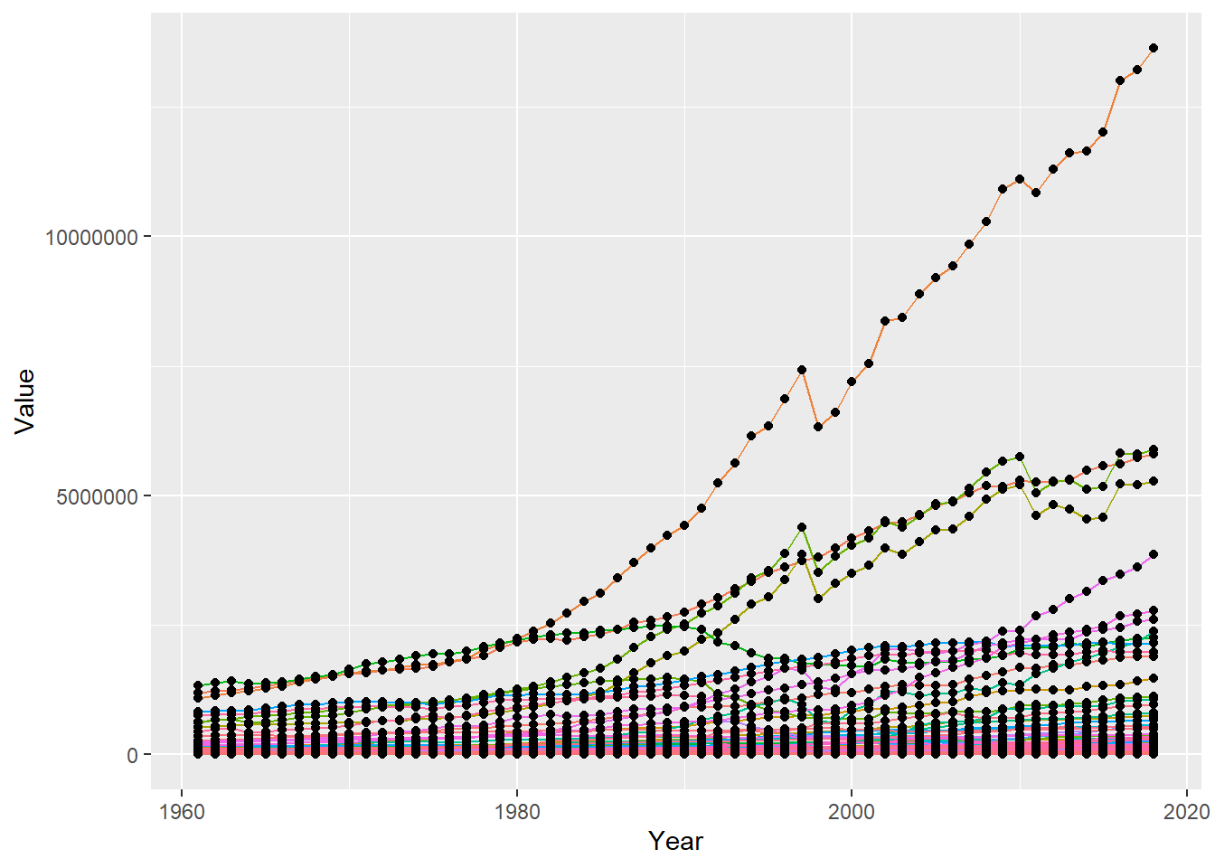

We see in this graph that there was a sharp decline in the global population of chickens from 1997-1998. After some research I believe this was due to the avian flu which gained traction during this time period.

https://www.nytimes.com/1997/12/29/world/chickens-killed-in-hong-kong-to-combat-flu.html

Provide Grouped Summary Statistics

Conduct some exploratory data analysis, using dplyr commands such as group_by(), select(), filter(), and summarise(). Find the central tendency (mean, median, mode) and dispersion (standard deviation, min/max/quantile) for different subgroups within the data set.

According to official data the average amount of chickens in 2018 per country was: (Note: if 1000 Head means this value is a grouping of a thousand then we would multiply by 1000 as done below)

Code

birdsData %>%
filter(`Flag Description` == "Official data",Year == 2018,Area!= "World") %>%
  group_by(Item)%>%
  summarise(MeanNumBirds = (mean(Value,na.rm= TRUE)*1000),sd=sd(Value,na.rm= TRUE))

# A tibble: 4 × 3
  Item                   MeanNumBirds      sd
  <chr>                         <dbl>   <dbl>
1 Chickens                 134517825. 357894.
2 Ducks                     10558815.  20605.
3 Geese and guinea fowls      885158.   1590.
4 Turkeys                   11933923.  47711.

An interesting comment here is how across each region the mean number of ducks and turkeys are relatively the same however the Standard deviation for the number of Turkeys is almost double that of ducks. I would think this is because in more of the developed world Turkeys are farmed over Ducks. With only a portion of the world farming turkeys and ducks naturally existing globally, this difference would make sense.

Minimum chickens, Aruba had no officially documented chickens in 1991 and 1992

Code

birdsData %>%
  filter(Item=="Chickens",Value == 0)

# A tibble: 2 × 14
  Domai…¹ Domain Area …² Area  Eleme…³ Element Item …⁴ Item  Year …⁵  Year Unit 
  <chr>   <chr>    <dbl> <chr>   <dbl> <chr>     <dbl> <chr>   <dbl> <dbl> <chr>
1 QA      Live …      22 Aruba    5112 Stocks     1057 Chic…    1991  1991 1000…
2 QA      Live …      22 Aruba    5112 Stocks     1057 Chic…    1992  1992 1000…
# … with 3 more variables: Value <dbl>, Flag <chr>, `Flag Description` <chr>,
#   and abbreviated variable names ¹`Domain Code`, ²`Area Code`,
#   ³`Element Code`, ⁴`Item Code`, ⁵`Year Code`

The maximum number of chickens in one area was Asia in 2018 with 13630958 1000 Heads of chickens

Code

birdsData %>%
  filter(Item=="Chickens", Area != "World")%>%
  slice_max(order_by = Value)

# A tibble: 1 × 14
  Domai…¹ Domain Area …² Area  Eleme…³ Element Item …⁴ Item  Year …⁵  Year Unit 
  <chr>   <chr>    <dbl> <chr>   <dbl> <chr>     <dbl> <chr>   <dbl> <dbl> <chr>
1 QA      Live …    5300 Asia     5112 Stocks     1057 Chic…    2018  2018 1000…
# … with 3 more variables: Value <dbl>, Flag <chr>, `Flag Description` <chr>,
#   and abbreviated variable names ¹`Domain Code`, ²`Area Code`,
#   ³`Element Code`, ⁴`Item Code`, ⁵`Year Code`

Explain and Interpret

Included throughout.