Code
library(tidyverse)
library(lubridate)
knitr::opts_chunk$set(echo = TRUE, warning=FALSE, message=FALSE)library(tidyverse)
library(lubridate)
knitr::opts_chunk$set(echo = TRUE, warning=FALSE, message=FALSE)For Homework 2 I found a dataset on Kaggle about Shark Attacks that I am reading in below using read_csv, renaming it to “shark” to make it easy to work with. I will then describe the dataset as well as what I am doing to tidy/mutate it to answer potential questions or points of analysis. The dataset I downloaded can be found here: https://www.kaggle.com/datasets/mysarahmadbhat/shark-attacks
My goal is to be able to describe some high level statistics about shark attacks in the USA since 2000.
shark <- read_csv("_data/shark attacks_abbybalintHW2.csv")
head(shark)
# A tibble: 6 × 22
Case Numbe…¹ Date Year Type Country Area Locat…² Activ…³ Name Sex Age
<chr> <chr> <dbl> <chr> <chr> <chr> <chr> <chr> <chr> <chr> <chr>
1 2017.06.11 6/11… 2017 Unpr… AUSTRA… West… Point … Body b… Paul… M 48
2 2017.06.10.b 6/10… 2017 Unpr… AUSTRA… Vict… Flinde… Surfing fema… F <NA>
3 2017.06.10.a 6/10… 2017 Unpr… USA Flor… Ponce … Surfing Brya… M 19
4 2017.06.07.R Repo… 2017 Unpr… UNITED… Sout… Bantha… Surfing Rich… M 30
5 2017.06.04 6/4/… 2017 Unpr… USA Flor… Middle… Spearf… Park… M <NA>
6 2017.06.02 6/2/… 2017 Unpr… BAHAMAS New … Athol … Snorke… Tiff… F 32
# … with 11 more variables: Injury <chr>, `Fatal (Y/N)` <chr>, Time <chr>,
# Species <chr>, `Investigator or Source` <chr>, pdf <chr>,
# `href formula` <chr>, href <chr>, `Case Number...20` <chr>,
# `Case Number...21` <chr>, `original order` <dbl>, and abbreviated variable
# names ¹`Case Number...1`, ²Location, ³ActivityThis dataset is from Kaggle and appears to likely be an aggregate of a few different data sources as it goes back to the late 1800’s all the way to 2017, including over 6,000 individual shark attacks. The data spans several countries. There is a variable titled “source” that describes where each individual attack was originally cited from. There are 22 variables, however many of them are different ways of describing a date, so it makes sense to choose the best column representative of date and remove some of the others. The other columns describe each shark attack with variables like location, activity, demos about the victim, injury type, and shark species.
sharknew <- shark %>%
select("Date":"Species", "original order")head(sharknew)# A tibble: 6 × 15
Date Year Type Country Area Locat…¹ Activ…² Name Sex Age Injury
<chr> <dbl> <chr> <chr> <chr> <chr> <chr> <chr> <chr> <chr> <chr>
1 6/11/17 2017 Unpr… AUSTRA… West… Point … Body b… Paul… M 48 No in…
2 6/10/17 2017 Unpr… AUSTRA… Vict… Flinde… Surfing fema… F <NA> No in…
3 6/10/17 2017 Unpr… USA Flor… Ponce … Surfing Brya… M 19 Lacer…
4 Reported 0… 2017 Unpr… UNITED… Sout… Bantha… Surfing Rich… M 30 Bruis…
5 6/4/17 2017 Unpr… USA Flor… Middle… Spearf… Park… M <NA> Lacer…
6 6/2/17 2017 Unpr… BAHAMAS New … Athol … Snorke… Tiff… F 32 Right…
# … with 4 more variables: `Fatal (Y/N)` <chr>, Time <chr>, Species <chr>,
# `original order` <dbl>, and abbreviated variable names ¹Location, ²Activitysharknew %>%
filter(`Country` == "USA", `Year` >= "2000") %>%
arrange(`original order`)# A tibble: 963 × 15
Date Year Type Country Area Locat…¹ Activ…² Name Sex Age Injury
<chr> <dbl> <chr> <chr> <chr> <chr> <chr> <chr> <chr> <chr> <chr>
1 6/22/05 2000 Boat USA Flor… Boca G… Fishin… boat… M <NA> No in…
2 2/21/00 2000 Unprovo… USA Flor… Rivier… <NA> male M 27 Right…
3 3/1/00 2000 Unprovo… USA Loui… Midnig… Spearf… Kurt… M 39 No in…
4 3/24/00 2000 Unprovo… USA Flor… Florid… Surfing Barr… M 37 Left …
5 3/26/00 2000 Unprovo… USA Flor… Juno B… Boogie… Heat… F 14 Right…
6 3/31/00 2000 Unprovo… USA Flor… Santa … Fishing Dave… M <NA> No In…
7 4/9/00 2000 Unprovo… USA Flor… Munici… Boogie… teen M <NA> Punct…
8 4/14/00 2000 Unprovo… USA Flor… On the… Walking Adam… M 34 Left …
9 6/2/00 2000 Unprovo… USA Flor… 27th A… Snorke… Bria… M 13 Right…
10 6/9/00 2000 Unprovo… USA Alab… Gulf S… Swimmi… Chuc… M 44 Right…
# … with 953 more rows, 4 more variables: `Fatal (Y/N)` <chr>, Time <chr>,
# Species <chr>, `original order` <dbl>, and abbreviated variable names
# ¹Location, ²Activitysharknew %>%
filter(`Country` == "USA", `Year` >= "2000") %>%
arrange(`original order`) %>%
separate(col=`Location`, into=c("Description" , "County"), sep = ",") %>%
rename(State = `Area`)# A tibble: 963 × 16
Date Year Type Country State Descr…¹ County Activ…² Name Sex Age
<chr> <dbl> <chr> <chr> <chr> <chr> <chr> <chr> <chr> <chr> <chr>
1 6/22/05 2000 Boat USA Flor… Boca G… " Lee… Fishin… boat… M <NA>
2 2/21/00 2000 Unprovo… USA Flor… Rivier… " Pal… <NA> male M 27
3 3/1/00 2000 Unprovo… USA Loui… Midnig… <NA> Spearf… Kurt… M 39
4 3/24/00 2000 Unprovo… USA Flor… Florid… " Bre… Surfing Barr… M 37
5 3/26/00 2000 Unprovo… USA Flor… Juno B… " Pal… Boogie… Heat… F 14
6 3/31/00 2000 Unprovo… USA Flor… Santa … <NA> Fishing Dave… M <NA>
7 4/9/00 2000 Unprovo… USA Flor… Munici… " Riv… Boogie… teen M <NA>
8 4/14/00 2000 Unprovo… USA Flor… On the… " Vol… Walking Adam… M 34
9 6/2/00 2000 Unprovo… USA Flor… 27th A… " New… Snorke… Bria… M 13
10 6/9/00 2000 Unprovo… USA Alab… Gulf S… " Bal… Swimmi… Chuc… M 44
# … with 953 more rows, 5 more variables: Injury <chr>, `Fatal (Y/N)` <chr>,
# Time <chr>, Species <chr>, `original order` <dbl>, and abbreviated variable
# names ¹Description, ²Activitysharknew %>%
filter(`Country` == "USA", `Year` >= "2000") %>%
arrange(`original order`) %>%
separate(col=`Location`, into=c("Description" , "County"), sep = ",") %>%
rename(State = `Area`) %>%
mutate(`AgeRanges` = dplyr::case_when(
`Age` >= 18 & `Age` <= 24 ~ "18-24",
`Age` >= 25 & `Age` <= 34 ~ "25-34",
`Age` >= 35 & `Age` <= 44 ~ "18-44",
`Age` >= 45 & `Age` <= 54 ~ "18-54",
`Age` >= 55 ~ "55+" ))# A tibble: 963 × 17
Date Year Type Country State Descr…¹ County Activ…² Name Sex Age
<chr> <dbl> <chr> <chr> <chr> <chr> <chr> <chr> <chr> <chr> <chr>
1 6/22/05 2000 Boat USA Flor… Boca G… " Lee… Fishin… boat… M <NA>
2 2/21/00 2000 Unprovo… USA Flor… Rivier… " Pal… <NA> male M 27
3 3/1/00 2000 Unprovo… USA Loui… Midnig… <NA> Spearf… Kurt… M 39
4 3/24/00 2000 Unprovo… USA Flor… Florid… " Bre… Surfing Barr… M 37
5 3/26/00 2000 Unprovo… USA Flor… Juno B… " Pal… Boogie… Heat… F 14
6 3/31/00 2000 Unprovo… USA Flor… Santa … <NA> Fishing Dave… M <NA>
7 4/9/00 2000 Unprovo… USA Flor… Munici… " Riv… Boogie… teen M <NA>
8 4/14/00 2000 Unprovo… USA Flor… On the… " Vol… Walking Adam… M 34
9 6/2/00 2000 Unprovo… USA Flor… 27th A… " New… Snorke… Bria… M 13
10 6/9/00 2000 Unprovo… USA Alab… Gulf S… " Bal… Swimmi… Chuc… M 44
# … with 953 more rows, 6 more variables: Injury <chr>, `Fatal (Y/N)` <chr>,
# Time <chr>, Species <chr>, `original order` <dbl>, AgeRanges <chr>, and
# abbreviated variable names ¹Description, ²Activitysharkfinal <- sharknewsharknew %>%
filter(`Country` == "USA", `Year` >= "2000") %>%
arrange(`original order`) %>%
separate(col=`Location`, into=c("Description" , "County"), sep = ",") %>%
rename(State = `Area`) %>%
mutate(`AgeRanges` = dplyr::case_when(
`Age` >= 18 & `Age` <= 24 ~ "18-24",
`Age` >= 25 & `Age` <= 34 ~ "25-34",
`Age` >= 35 & `Age` <= 44 ~ "18-44",
`Age` >= 45 & `Age` <= 54 ~ "18-54",
`Age` >= 55 ~ "55+" )) %>%
ggplot(aes(`Type`)) + geom_bar()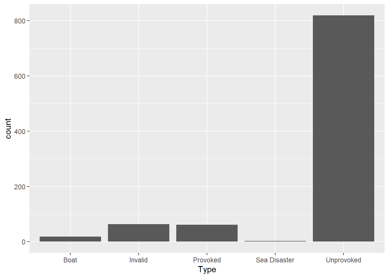
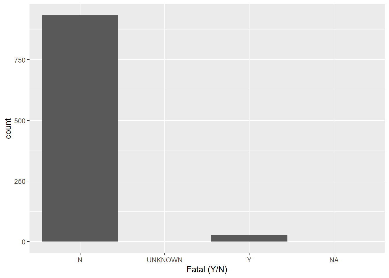
sharknew %>%
  filter(`Country` == "USA", `Year` >= "2000") %>%
arrange(`original order`) %>%
separate(col=`Location`, into=c("Description" , "County"), sep = ",") %>%
rename(State = `Area`) %>%
mutate(`AgeRanges` = dplyr::case_when(
`Age` >= 18 & `Age` <= 24 ~ "18-24",
`Age` >= 25 & `Age` <= 34 ~ "25-34",
`Age` >= 35 & `Age` <= 44 ~ "18-44",
`Age` >= 45 & `Age` <= 54 ~ "18-54",
`Age` >= 55 ~ "55+" )) %>%
ggplot(aes(`Fatal (Y/N)`)) + geom_bar()