Code
library(tidyverse)

knitr::opts_chunk$set(echo = TRUE, warning=FALSE, message=FALSE)Homework 2
For this homework, your goal is to read in a more complicated dataset. Please use the category tag “hw2” as well as a tag for the dataset you choose to use. Read in a dataset from the _data folder in the course blog repository, or choose your own data. If you decide to use one of the datasets we have provided, please use a challenging dataset - check with us if you are not sure. Clean the data as needed using dplyr and related tidyverse packages. Provide a narrative about the data set (look it up if you aren’t sure what you have got) and the variables in your dataset, including what type of data each variable is. The goal of this step is to communicate in a visually appealing way to non-experts - not to replicate r-code. Identify potential research questions that your data set can help answer.
library(tidyverse)
knitr::opts_chunk$set(echo = TRUE, warning=FALSE, message=FALSE)The dataset that I have chosen to work is FedFunds data set which gives insights about the economics, inflation etc..,
we initially read the Fed funds data that is already present in the data folder
library(readr)
FedFundsRate <- read_csv("_data/FedFundsRate.csv")
View(FedFundsRate)while we initially see the data, we see that there are a lot of NA’ s in the data in the initial glance. But to understand more about the data, we need to further analyse it.
Extracting the column names
colnames(FedFundsRate) [1] "Year" "Month"
[3] "Day" "Federal Funds Target Rate"
[5] "Federal Funds Upper Target" "Federal Funds Lower Target"
[7] "Effective Federal Funds Rate" "Real GDP (Percent Change)"
[9] "Unemployment Rate" "Inflation Rate" Getting the size of the data
dim(FedFundsRate)[1] 904 10We see that there about 904 rows and 10 columns in the dataset
let’s visualize the sample data
head(FedFundsRate)# A tibble: 6 × 10
Year Month Day Federal Fu…¹ Feder…² Feder…³ Effec…⁴ Real …⁵ Unemp…⁶ Infla…⁷
<dbl> <dbl> <dbl> <dbl> <dbl> <dbl> <dbl> <dbl> <dbl> <dbl>
1 1954 7 1 NA NA NA 0.8 4.6 5.8 NA
2 1954 8 1 NA NA NA 1.22 NA 6 NA
3 1954 9 1 NA NA NA 1.06 NA 6.1 NA
4 1954 10 1 NA NA NA 0.85 8 5.7 NA
5 1954 11 1 NA NA NA 0.83 NA 5.3 NA
6 1954 12 1 NA NA NA 1.28 NA 5 NA
# … with abbreviated variable names ¹`Federal Funds Target Rate`,
# ²`Federal Funds Upper Target`, ³`Federal Funds Lower Target`,
# ⁴`Effective Federal Funds Rate`, ⁵`Real GDP (Percent Change)`,
# ⁶`Unemployment Rate`, ⁷`Inflation Rate`let’s get the summary of the data in the firstplace to clean the data.
summary(FedFundsRate) Year Month Day Federal Funds Target Rate
Min. :1954 Min. : 1.000 Min. : 1.000 Min. : 1.000
1st Qu.:1973 1st Qu.: 4.000 1st Qu.: 1.000 1st Qu.: 3.750
Median :1988 Median : 7.000 Median : 1.000 Median : 5.500
Mean :1987 Mean : 6.598 Mean : 3.598 Mean : 5.658
3rd Qu.:2001 3rd Qu.:10.000 3rd Qu.: 1.000 3rd Qu.: 7.750
Max. :2017 Max. :12.000 Max. :31.000 Max. :11.500
NA's :442
Federal Funds Upper Target Federal Funds Lower Target
Min. :0.2500 Min. :0.0000
1st Qu.:0.2500 1st Qu.:0.0000
Median :0.2500 Median :0.0000
Mean :0.3083 Mean :0.0583
3rd Qu.:0.2500 3rd Qu.:0.0000
Max. :1.0000 Max. :0.7500
NA's :801 NA's :801
Effective Federal Funds Rate Real GDP (Percent Change) Unemployment Rate
Min. : 0.070 Min. :-10.000 Min. : 3.400
1st Qu.: 2.428 1st Qu.: 1.400 1st Qu.: 4.900
Median : 4.700 Median : 3.100 Median : 5.700
Mean : 4.911 Mean : 3.138 Mean : 5.979
3rd Qu.: 6.580 3rd Qu.: 4.875 3rd Qu.: 7.000
Max. :19.100 Max. : 16.500 Max. :10.800
NA's :152 NA's :654 NA's :152
Inflation Rate
Min. : 0.600
1st Qu.: 2.000
Median : 2.800
Mean : 3.733
3rd Qu.: 4.700
Max. :13.600
NA's :194 Looking at the summary we see that there are a lot of NA’s present in the data in almost all the columns except for Year,Month,date.Inorder to clean the data, we must drop all the NA’s present in the data.
cleaned_fed_funds <- na.omit(FedFundsRate)
cleaned_fed_funds
# A tibble: 0 × 10
# … with 10 variables: Year <dbl>, Month <dbl>, Day <dbl>,
# Federal Funds Target Rate <dbl>, Federal Funds Upper Target <dbl>,
# Federal Funds Lower Target <dbl>, Effective Federal Funds Rate <dbl>,
# Real GDP (Percent Change) <dbl>, Unemployment Rate <dbl>,
# Inflation Rate <dbl>A new data frame with the name of cleaned_fed_funds is created after dropping all the NA’s.
if we drop all the NA’s then we are getting no rows in the data set.Let’s try an other way of dropping na’s
cleaned_fed_funds1 <- FedFundsRate %>%
  drop_na(Year,`Federal Funds Target Rate`,`Federal Funds Upper Target`,`Federal Funds Lower Target`,`Effective Federal Funds Rate`,`Unemployment Rate`,`Inflation Rate`)
cleaned_fed_funds1
# A tibble: 0 × 10
# … with 10 variables: Year <dbl>, Month <dbl>, Day <dbl>,
# Federal Funds Target Rate <dbl>, Federal Funds Upper Target <dbl>,
# Federal Funds Lower Target <dbl>, Effective Federal Funds Rate <dbl>,
# Real GDP (Percent Change) <dbl>, Unemployment Rate <dbl>,
# Inflation Rate <dbl>So inorder to retain the dataset, let’s drop NA’s from those of the columns that we would actually like to visualize or consider them important.
cleaned_fed_funds1 <- FedFundsRate %>%
  drop_na(`Effective Federal Funds Rate`,`Unemployment Rate`,`Inflation Rate`,`Real GDP (Percent Change)`)
cleaned_fed_funds1
# A tibble: 236 × 10
Year Month Day Federal F…¹ Feder…² Feder…³ Effec…⁴ Real …⁵ Unemp…⁶ Infla…⁷
<dbl> <dbl> <dbl> <dbl> <dbl> <dbl> <dbl> <dbl> <dbl> <dbl>
1 1958 1 1 NA NA NA 2.72 -10 5.8 3.2
2 1958 4 1 NA NA NA 1.26 2.6 7.4 2.4
3 1958 7 1 NA NA NA 0.68 9.6 7.5 2.4
4 1958 10 1 NA NA NA 1.8 9.7 6.7 1.7
5 1959 1 1 NA NA NA 2.48 7.7 6 1.7
6 1959 4 1 NA NA NA 2.96 10.1 5.2 1.7
7 1959 7 1 NA NA NA 3.47 -0.8 5.1 2
8 1959 10 1 NA NA NA 3.98 1.6 5.7 2.7
9 1960 1 1 NA NA NA 3.99 9.2 5.2 2
10 1960 4 1 NA NA NA 3.92 -1.5 5.2 2
# … with 226 more rows, and abbreviated variable names
# ¹`Federal Funds Target Rate`, ²`Federal Funds Upper Target`,
# ³`Federal Funds Lower Target`, ⁴`Effective Federal Funds Rate`,
# ⁵`Real GDP (Percent Change)`, ⁶`Unemployment Rate`, ⁷`Inflation Rate`summary(cleaned_fed_funds1) Year Month Day Federal Funds Target Rate
Min. :1958 Min. : 1.00 Min. :1 Min. : 1.000
1st Qu.:1972 1st Qu.: 3.25 1st Qu.:1 1st Qu.: 3.750
Median :1987 Median : 5.50 Median :1 Median : 5.250
Mean :1987 Mean : 5.50 Mean :1 Mean : 5.407
3rd Qu.:2002 3rd Qu.: 7.75 3rd Qu.:1 3rd Qu.: 7.000
Max. :2016 Max. :10.00 Max. :1 Max. :11.000
NA's :131
Federal Funds Upper Target Federal Funds Lower Target
Min. :0.2500 Min. :0.00000
1st Qu.:0.2500 1st Qu.:0.00000
Median :0.2500 Median :0.00000
Mean :0.2812 Mean :0.03125
3rd Qu.:0.2500 3rd Qu.:0.00000
Max. :0.5000 Max. :0.25000
NA's :204 NA's :204
Effective Federal Funds Rate Real GDP (Percent Change) Unemployment Rate
Min. : 0.070 Min. :-10.000 Min. : 3.400
1st Qu.: 2.655 1st Qu.: 1.400 1st Qu.: 5.000
Median : 4.845 Median : 3.100 Median : 5.700
Mean : 5.084 Mean : 3.116 Mean : 6.074
3rd Qu.: 6.875 3rd Qu.: 4.800 3rd Qu.: 7.100
Max. :19.080 Max. : 16.500 Max. :10.400
Inflation Rate
Min. : 0.600
1st Qu.: 2.000
Median : 2.800
Mean : 3.740
3rd Qu.: 4.725
Max. :13.000
cleaned_fed_funds1 <-cleaned_fed_funds1%>%
  mutate_at(vars(colnames(cleaned_fed_funds1)[0:10]), function(x)as.numeric(x))
glimpse(cleaned_fed_funds1)
Rows: 236
Columns: 10
$ Year <dbl> 1958, 1958, 1958, 1958, 1959, 1959, 195…
$ Month <dbl> 1, 4, 7, 10, 1, 4, 7, 10, 1, 4, 7, 10, …
$ Day <dbl> 1, 1, 1, 1, 1, 1, 1, 1, 1, 1, 1, 1, 1, …
$ `Federal Funds Target Rate` <dbl> NA, NA, NA, NA, NA, NA, NA, NA, NA, NA,…
$ `Federal Funds Upper Target` <dbl> NA, NA, NA, NA, NA, NA, NA, NA, NA, NA,…
$ `Federal Funds Lower Target` <dbl> NA, NA, NA, NA, NA, NA, NA, NA, NA, NA,…
$ `Effective Federal Funds Rate` <dbl> 2.72, 1.26, 0.68, 1.80, 2.48, 2.96, 3.4…
$ `Real GDP (Percent Change)` <dbl> -10.0, 2.6, 9.6, 9.7, 7.7, 10.1, -0.8, …
$ `Unemployment Rate` <dbl> 5.8, 7.4, 7.5, 6.7, 6.0, 5.2, 5.1, 5.7,…
$ `Inflation Rate` <dbl> 3.2, 2.4, 2.4, 1.7, 1.7, 1.7, 2.0, 2.7,…a <- cleaned_fed_funds1%>%
group_by(Year)
a# A tibble: 236 × 10
# Groups: Year [59]
Year Month Day Federal F…¹ Feder…² Feder…³ Effec…⁴ Real …⁵ Unemp…⁶ Infla…⁷
<dbl> <dbl> <dbl> <dbl> <dbl> <dbl> <dbl> <dbl> <dbl> <dbl>
1 1958 1 1 NA NA NA 2.72 -10 5.8 3.2
2 1958 4 1 NA NA NA 1.26 2.6 7.4 2.4
3 1958 7 1 NA NA NA 0.68 9.6 7.5 2.4
4 1958 10 1 NA NA NA 1.8 9.7 6.7 1.7
5 1959 1 1 NA NA NA 2.48 7.7 6 1.7
6 1959 4 1 NA NA NA 2.96 10.1 5.2 1.7
7 1959 7 1 NA NA NA 3.47 -0.8 5.1 2
8 1959 10 1 NA NA NA 3.98 1.6 5.7 2.7
9 1960 1 1 NA NA NA 3.99 9.2 5.2 2
10 1960 4 1 NA NA NA 3.92 -1.5 5.2 2
# … with 226 more rows, and abbreviated variable names
# ¹`Federal Funds Target Rate`, ²`Federal Funds Upper Target`,
# ³`Federal Funds Lower Target`, ⁴`Effective Federal Funds Rate`,
# ⁵`Real GDP (Percent Change)`, ⁶`Unemployment Rate`, ⁷`Inflation Rate`table(cleaned_fed_funds1$Year)
1958 1959 1960 1961 1962 1963 1964 1965 1966 1967 1968 1969 1970 1971 1972 1973
   4    4    4    4    4    4    4    4    4    4    4    4    4    4    4    4
1974 1975 1976 1977 1978 1979 1980 1981 1982 1983 1984 1985 1986 1987 1988 1989
   4    4    4    4    4    4    4    4    4    4    4    4    4    4    4    4
1990 1991 1992 1993 1994 1995 1996 1997 1998 1999 2000 2001 2002 2003 2004 2005
   4    4    4    4    4    4    4    4    4    4    4    4    4    4    4    4
2006 2007 2008 2009 2010 2011 2012 2013 2014 2015 2016
   4    4    4    4    4    4    4    4    4    4    4
we see that there are a range of years, from 1958-2016
print(summarytools::dfSummary(cleaned_fed_funds1,
                        varnumbers = FALSE,
                        plain.ascii  = FALSE,
                        style        = "grid",
                        graph.magnif = 0.70,
                        valid.col    = FALSE),
      method = 'render',
table.classes = 'table-condensed')| Variable | Stats / Values | Freqs (% of Valid) | Graph | Missing | ||||||||||||||||||||||||||||
|---|---|---|---|---|---|---|---|---|---|---|---|---|---|---|---|---|---|---|---|---|---|---|---|---|---|---|---|---|---|---|---|---|
| Year [numeric] |
|
59 distinct values |  |
0 (0.0%) | ||||||||||||||||||||||||||||
| Month [numeric] |
|
|
 |
0 (0.0%) | ||||||||||||||||||||||||||||
| Day [numeric] | 1 distinct value |
|
 |
0 (0.0%) | ||||||||||||||||||||||||||||
| Federal Funds Target Rate [numeric] |
|
42 distinct values |  |
131 (55.5%) | ||||||||||||||||||||||||||||
| Federal Funds Upper Target [numeric] |
|
2 distinct values |  |
204 (86.4%) | ||||||||||||||||||||||||||||
| Federal Funds Lower Target [numeric] |
|
2 distinct values | |
204 (86.4%) | ||||||||||||||||||||||||||||
| Effective Federal Funds Rate [numeric] |
|
193 distinct values |  |
0 (0.0%) | ||||||||||||||||||||||||||||
| Real GDP (Percent Change) [numeric] |
|
110 distinct values |  |
0 (0.0%) | ||||||||||||||||||||||||||||
| Unemployment Rate [numeric] |
|
62 distinct values |  |
0 (0.0%) | ||||||||||||||||||||||||||||
| Inflation Rate [numeric] |
|
75 distinct values |  |
0 (0.0%) |
Generated by summarytools 1.0.1 (R version 4.2.1)
2022-12-20
Now we can look at the summary and get few insights from the data regarding the data type of the columns,statistical analysis, frequency of the data etc..,
Understanding year-wise GDP metrics
cleaned_fed_funds1$Year<-as.factor(cleaned_fed_funds1$Year)
cleaned_fed_funds1 %>%
  group_by(Year) %>%
  summarise(GDP_min=min(`Real GDP (Percent Change)`),GDP_max=max(`Real GDP (Percent Change)`),GDP_mean=mean(`Real GDP (Percent Change)`), .groups = 'keep') %>%
  arrange(desc(Year)) %>%
  print(n = 100)
# A tibble: 59 × 4
# Groups: Year [59]
Year GDP_min GDP_max GDP_mean
<fct> <dbl> <dbl> <dbl>
1 2016 0.8 3.5 1.9
2 2015 0.9 2.6 1.88
3 2014 -1.2 5 2.52
4 2013 0.8 4 2.68
5 2012 0.1 2.7 1.3
6 2011 -1.5 4.6 1.7
7 2010 1.7 3.9 2.7
8 2009 -5.4 3.9 -0.175
9 2008 -8.2 2 -2.7
10 2007 0.2 3.1 1.85
11 2006 0.4 4.9 2.43
12 2005 2.1 4.3 3.02
13 2004 2.3 3.7 3.12
14 2003 2.1 6.9 4.4
15 2002 0.3 3.7 2.05
16 2001 -1.3 2.1 0.2
17 2000 0.5 7.8 2.95
18 1999 3.2 7.1 4.68
19 1998 3.9 6.7 4.97
20 1997 3.1 6.2 4.4
21 1996 2.7 7.2 4.47
22 1995 1.4 3.5 2.3
23 1994 2.4 5.6 4.15
24 1993 0.8 5.4 2.65
25 1992 3.9 4.8 4.32
26 1991 -1.9 3.1 1.23
27 1990 -3.4 4.5 0.7
28 1989 0.9 4.1 2.8
29 1988 2.3 5.4 3.85
30 1987 2.8 6.8 4.47
31 1986 1.9 4.1 2.97
32 1985 3 6.4 4.28
33 1984 3.2 8.2 5.65
34 1983 5.3 9.4 7.82
35 1982 -6.5 2.2 -1.32
36 1981 -4.6 8.5 1.43
37 1980 -7.9 7.6 0.100
38 1979 0.5 2.9 1.3
39 1978 1.4 16.5 6.85
40 1977 0 8.1 5.03
41 1976 2.1 9.3 4.38
42 1975 -4.7 6.8 2.68
43 1974 -3.8 1.1 -1.9
44 1973 -2.2 10.2 4.1
45 1972 3.7 9.6 6.88
46 1971 1.2 11.1 4.45
47 1970 -4 3.6 -0.1
48 1969 -1.7 6.4 2.12
49 1968 1.8 8.4 5
50 1967 0.3 3.7 2.68
51 1966 1.6 10.2 4.55
52 1965 5.6 10.2 8.5
53 1964 1.4 8.9 5.15
54 1963 2.9 8 5.18
55 1962 1.6 7.4 4.32
56 1961 2.7 8.3 6.35
57 1960 -4.8 9.2 0.975
58 1959 -0.8 10.1 4.65
59 1958 -10 9.7 2.97 Lets see how un employement rate is being affected with year
ggplot(cleaned_fed_funds1) +
  aes(x = `Inflation Rate`, y = `Unemployment Rate`) +
  geom_point(colour = "#69b3a2") +
  theme_minimal()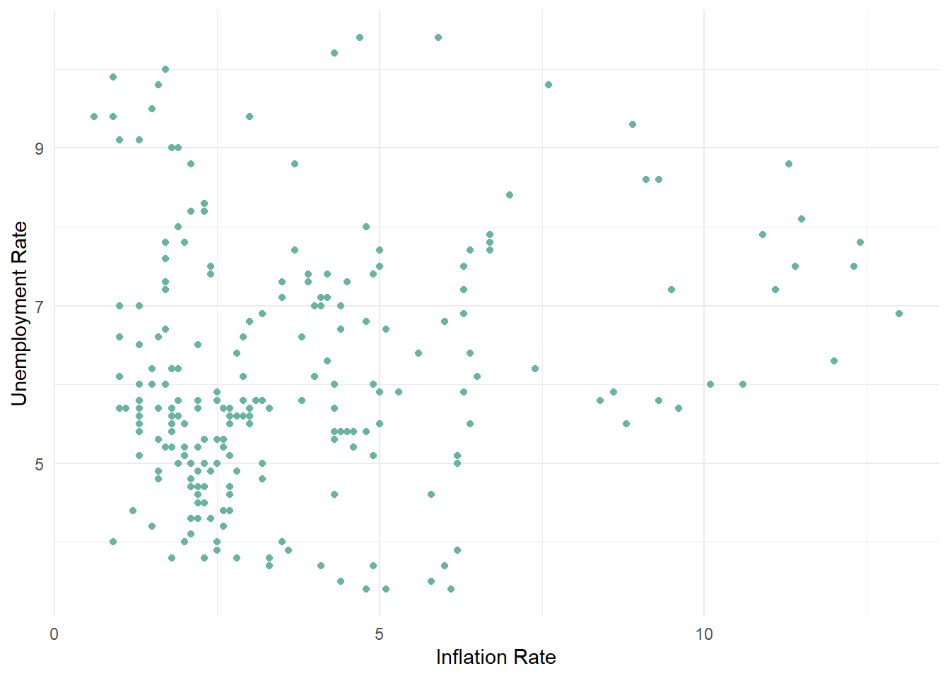
a <- cleaned_fed_funds1 %>%
  select(Year, `Real GDP (Percent Change)`, `Inflation Rate`) %>%
  gather(key = "variable", value = "value", -Year)
ggplot(a, aes(x =`Year`, y = value)) +
  geom_line(aes(color = variable, linetype = variable)) +
  scale_color_manual(values = c("darkred", "steelblue"))+labs(
  title = "Inflation and gdp change by Year",
  y = "Variable Rates", x = "Year")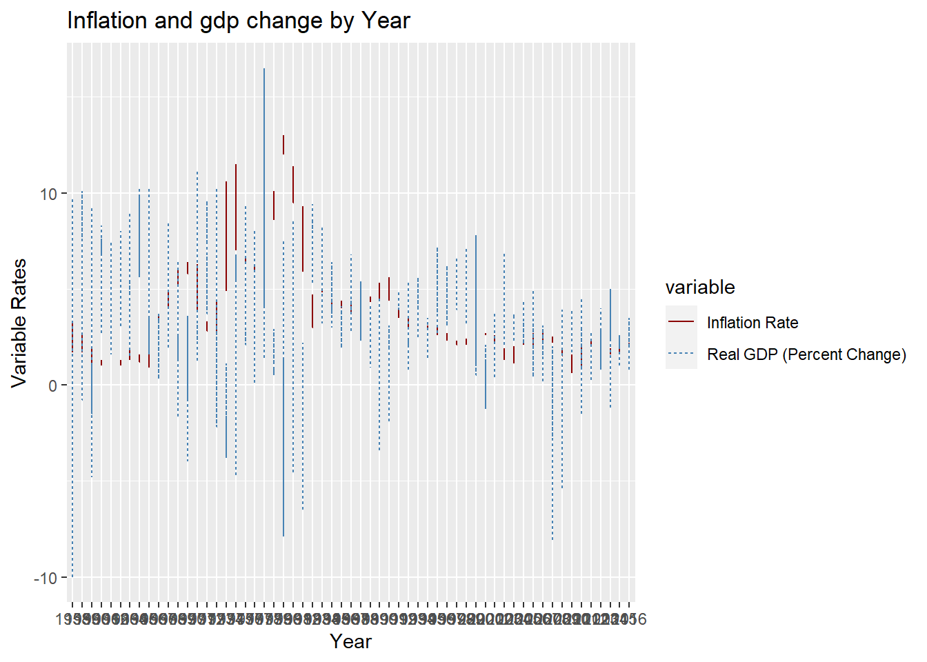
The entire data set talks about the economic stability of a country.
The data can answer questions about how the un employment and inflation rates are inter related, how the GDP change is changing year over year.
we can also see the relation between inflation rates, GDP Change as well. various combinations of column data’s can be considered and worked over.