library(tidyverse)
library(ggplot2)

knitr::opts_chunk$set(echo = TRUE, warning=FALSE, message=FALSE)
Challenge 5
challenge_5
railroads
cereal
air_bnb
pathogen_cost
australian_marriage
public_schools
usa_households
Introduction to Visualization
Challenge Overview
Today’s challenge is to:
- read in a data set, and describe the data set using both words and any supporting information (e.g., tables, etc)
- tidy data (as needed, including sanity checks)
- mutate variables as needed (including sanity checks)
- create at least two univariate visualizations
- try to make them “publication” ready
- Explain why you choose the specific graph type
- Create at least one bivariate visualization
- try to make them “publication” ready
- Explain why you choose the specific graph type
R Graph Gallery is a good starting point for thinking about what information is conveyed in standard graph types, and includes example R code.
(be sure to only include the category tags for the data you use!)
Read in data
Read in one (or more) of the following datasets, using the correct R package and command.
- cereal.csv ⭐
- Total_cost_for_top_15_pathogens_2018.xlsx ⭐
- Australian Marriage ⭐⭐
- AB_NYC_2019.csv ⭐⭐⭐
- StateCounty2012.xls ⭐⭐⭐
- Public School Characteristics ⭐⭐⭐⭐
- USA Households ⭐⭐⭐⭐⭐
NYC_data <- read_csv("_data/AB_NYC_2019.csv")
NYC_data
# A tibble: 48,895 × 16
id name host_id host_…¹ neigh…² neigh…³ latit…⁴ longi…⁵ room_…⁶ price
<dbl> <chr> <dbl> <chr> <chr> <chr> <dbl> <dbl> <chr> <dbl>
1 2539 Clean & … 2787 John Brookl… Kensin… 40.6 -74.0 Privat… 149
2 2595 Skylit M… 2845 Jennif… Manhat… Midtown 40.8 -74.0 Entire… 225
3 3647 THE VILL… 4632 Elisab… Manhat… Harlem 40.8 -73.9 Privat… 150
4 3831 Cozy Ent… 4869 LisaRo… Brookl… Clinto… 40.7 -74.0 Entire… 89
5 5022 Entire A… 7192 Laura Manhat… East H… 40.8 -73.9 Entire… 80
6 5099 Large Co… 7322 Chris Manhat… Murray… 40.7 -74.0 Entire… 200
7 5121 BlissArt… 7356 Garon Brookl… Bedfor… 40.7 -74.0 Privat… 60
8 5178 Large Fu… 8967 Shunic… Manhat… Hell's… 40.8 -74.0 Privat… 79
9 5203 Cozy Cle… 7490 MaryEl… Manhat… Upper … 40.8 -74.0 Privat… 79
10 5238 Cute & C… 7549 Ben Manhat… Chinat… 40.7 -74.0 Entire… 150
# … with 48,885 more rows, 6 more variables: minimum_nights <dbl>,
# number_of_reviews <dbl>, last_review <date>, reviews_per_month <dbl>,
# calculated_host_listings_count <dbl>, availability_365 <dbl>, and
# abbreviated variable names ¹host_name, ²neighbourhood_group,
# ³neighbourhood, ⁴latitude, ⁵longitude, ⁶room_typeBriefly describe the data
This dataset is about different AirBNB properties listed in the New York City, in year 2019 and includes around 49000 and 16 columns. It includes data about each property’s host name, neighborhood and the neighborhood group, property type, price, and location.
Tidy Data (as needed)
There are a few columns with null values and I will be tidying data for those columns. I noticed that each row has a unique id which eliminates the possibility of having duplicate records and hence no tidying is needed in that respect.
table(NYC_data$reviews_per_month)
 0.01  0.02  0.03  0.04  0.05  0.06  0.07  0.08  0.09   0.1  0.11  0.12  0.13
   42   919   804   655   893   579   466   596   593   457   539   413   463
 0.14  0.15  0.16  0.17  0.18  0.19   0.2  0.21  0.22  0.23  0.24  0.25  0.26
  399   374   667   321   305   357   276   343   318   289   266   290   305
 0.27  0.28  0.29   0.3  0.31  0.32  0.33  0.34  0.35  0.36  0.37  0.38  0.39
  277   264   229   250   248   280   223   165   174   208   201   217   187
  0.4  0.41  0.42  0.43  0.44  0.45  0.46  0.47  0.48  0.49   0.5  0.51  0.52
  167   186   227   183   160   178   175   182   168   144   132   114   152
 0.53  0.54  0.55  0.56  0.57  0.58  0.59   0.6  0.61  0.62  0.63  0.64  0.65
  163   117   149   125   125   146   146   112   130   105   143   111   136
 0.66  0.67  0.68  0.69   0.7  0.71  0.72  0.73  0.74  0.75  0.76  0.77  0.78
  105   112   131    92   131   118    78   112    98   101   114   143    97
 0.79   0.8  0.81  0.82  0.83  0.84  0.85  0.86  0.87  0.88  0.89   0.9  0.91
  110    98   123    97    92    80   111    78    92    85    69    87   106
 0.92  0.93  0.94  0.95  0.96  0.97  0.98  0.99     1  1.01  1.02  1.03  1.04
   77    87   103    87    83    79    64    74   893    58    66    73    68
 1.05  1.06  1.07  1.08  1.09   1.1  1.11  1.12  1.13  1.14  1.15  1.16  1.17
   88    83    64    62    63    67    88    67    78    74    90    51    66
 1.18  1.19   1.2  1.21  1.22  1.23  1.24  1.25  1.26  1.27  1.28  1.29   1.3
   81    58    69    56    73    64    56    80    63    67    69    62    72
 1.31  1.32  1.33  1.34  1.35  1.36  1.37  1.38  1.39   1.4  1.41  1.42  1.43
   51    54    77    64    45    84    49    59    47    84    66    53    50
 1.44  1.45  1.46  1.47  1.48  1.49   1.5  1.51  1.52  1.53  1.54  1.55  1.56
   46    50    70    50    42    51    57    64    54    61    46    57    51
 1.57  1.58  1.59   1.6  1.61  1.62  1.63  1.64  1.65  1.66  1.67  1.68  1.69
   63    70    40    46    49    65    47    49    65    39    65    55    48
  1.7  1.71  1.72  1.73  1.74  1.75  1.76  1.77  1.78  1.79   1.8  1.81  1.82
   53    52    45    66    40    37    75    35    53    48    61    48    61
 1.83  1.84  1.85  1.86  1.87  1.88  1.89   1.9  1.91  1.92  1.93  1.94  1.95
   55    58    44    40    34    70    45    65    46    44    36    57    45
 1.96  1.97  1.98  1.99     2  2.01  2.02  2.03  2.04  2.05  2.06  2.07  2.08
   54    40    34    37   406    38    47    45    38    39    40    60    41
 2.09   2.1  2.11  2.12  2.13  2.14  2.15  2.16  2.17  2.18  2.19   2.2  2.21
   50    37    45    36    41    42    32    34    39    39    43    38    42
 2.22  2.23  2.24  2.25  2.26  2.27  2.28  2.29   2.3  2.31  2.32  2.33  2.34
   54    52    36    32    70    39    43    40    32    66    36    36    57
 2.35  2.36  2.37  2.38  2.39   2.4  2.41  2.42  2.43  2.44  2.45  2.46  2.47
   53    42    43    53    40    37    20    50    46    43    39    35    42
 2.48  2.49   2.5  2.51  2.52  2.53  2.54  2.55  2.56  2.57  2.58  2.59   2.6
   44    34    69    31    35    35    50    48    40    40    36    42    33
 2.61  2.62  2.63  2.64  2.65  2.66  2.67  2.68  2.69   2.7  2.71  2.72  2.73
   33    23    58    35    38    37    44    36    37    42    28    19    54
 2.74  2.75  2.76  2.77  2.78  2.79   2.8  2.81  2.82  2.83  2.84  2.85  2.86
   39    39    28    22    36    56    36    45    38    44    36    24    28
 2.87  2.88  2.89   2.9  2.91  2.92  2.93  2.94  2.95  2.96  2.97  2.98  2.99
   45    50    33    30    19    36    29    19    32    35    31    30    33
    3  3.01  3.02  3.03  3.04  3.05  3.06  3.07  3.08  3.09   3.1  3.11  3.12
  222    29    27    20    43    27    28    32    31    30    36    30    18
 3.13  3.14  3.15  3.16  3.17  3.18  3.19   3.2  3.21  3.22  3.23  3.24  3.25
   41    30    20    34    42    34    41    24    36    29    24    29    27
 3.26  3.27  3.28  3.29   3.3  3.31  3.32  3.33  3.34  3.35  3.36  3.37  3.38
   29    30    33    23    26    35    24    52    26    22    24    28    28
 3.39   3.4  3.41  3.42  3.43  3.44  3.45  3.46  3.47  3.48  3.49   3.5  3.51
   17    31    20    37    21    28    26    27    24    16    20    27    24
 3.52  3.53  3.54  3.55  3.56  3.57  3.58  3.59   3.6  3.61  3.62  3.63  3.64
   26    38    15    26    17    18    21    30    21    26    20    30    27
 3.65  3.66  3.67  3.68  3.69   3.7  3.71  3.72  3.73  3.74  3.75  3.76  3.77
   26    26    23    25    30    25    22    26    16    17    42     8    15
 3.78  3.79   3.8  3.81  3.82  3.83  3.84  3.85  3.86  3.87  3.88  3.89   3.9
   21    28    28    10    18    14    14    26    22    16    26    16    20
 3.91  3.92  3.93  3.94  3.95  3.96  3.97  3.98  3.99     4  4.01  4.02  4.03
   19    14    29    23    22    17    22    17    12   130    16    16    16
 4.04  4.05  4.06  4.07  4.08  4.09   4.1  4.11  4.12  4.13  4.14  4.15  4.16
   22    18    18    21    18    25    21    15    18    17    19    20    16
 4.17  4.18  4.19   4.2  4.21  4.22  4.23  4.24  4.25  4.26  4.27  4.28  4.29
   20    16    21    15    27    14    17    13    18    19    13     4    40
  4.3  4.31  4.32  4.33  4.34  4.35  4.36  4.37  4.38  4.39   4.4  4.41  4.42
    6    13     8    15    19    15    23    16    17    10    13    11    11
 4.43  4.44  4.45  4.46  4.47  4.48  4.49   4.5  4.51  4.52  4.53  4.54  4.55
   16    24    13    13    17    17    18    19    12    20    13     8    20
 4.56  4.57  4.58  4.59   4.6  4.61  4.62  4.63  4.64  4.65  4.66  4.67  4.68
    7    17    23    17     7     5    26    13    12    13    15    13     8
 4.69   4.7  4.71  4.72  4.73  4.74  4.75  4.76  4.77  4.78  4.79   4.8  4.81
   20     6    10    10    17    16     7    12    13    13    13     9    11
 4.82  4.83  4.84  4.85  4.86  4.87  4.88  4.89   4.9  4.91  4.92  4.93  4.94
   14    10    10     6    13     7    11    12    10    10    10    18     9
 4.95  4.96  4.97  4.98  4.99     5  5.01  5.02  5.03  5.04  5.05  5.06  5.07
   10    12     9     7     4    85     6     8    11    10     8     8     5
 5.08  5.09   5.1  5.11  5.12  5.13  5.14  5.15  5.16  5.17  5.18  5.19   5.2
   12     6     7    14    11     7     7     4    10     9     6    11    12
 5.21  5.22  5.23  5.24  5.25  5.26  5.27  5.28  5.29   5.3  5.31  5.32  5.33
    4     9     6     5     8     9    11     9     7     5     9     5     7
 5.34  5.35  5.36  5.37  5.38  5.39   5.4  5.41  5.42  5.43  5.44  5.45  5.46
    8     9     4    16     9     8     7     5     9     5     7    19     4
 5.47  5.48  5.49   5.5  5.51  5.52  5.53  5.54  5.55  5.56  5.57  5.58  5.59
    4     2     7     8     6     3     5    10     4     8     4     6    10
  5.6  5.61  5.62  5.63  5.64  5.65  5.66  5.67  5.68  5.69   5.7  5.71  5.72
    5     6     6     8     6     8     4     5     5     5     7     6     1
 5.73  5.74  5.75  5.76  5.77  5.78  5.79   5.8  5.81  5.82  5.83  5.84  5.85
    7     8     5     1     4     8     6     5     8     7    11     4     3
 5.86  5.87  5.88  5.89   5.9  5.91  5.92  5.93  5.94  5.95  5.96  5.97  5.98
    3     8     7     5     6     5     8     3     5     9     3     4     4
 5.99     6  6.01  6.02  6.03  6.04  6.05  6.06  6.07  6.08  6.09   6.1  6.11
    4    39     2     4     5     1     5     1     5     5     4     6     5
 6.12  6.13  6.14  6.15  6.17  6.18  6.19   6.2  6.21  6.22  6.23  6.24  6.25
    3     5     2     3     2     4     8     4     4     4     8     1     4
 6.26  6.27  6.28  6.29   6.3  6.31  6.32  6.34  6.35  6.36  6.37  6.38  6.39
    2     2     3     1     3     5     7     3     4     5     3     6     1
  6.4  6.41  6.42  6.43  6.44  6.45  6.46  6.47  6.48  6.49   6.5  6.51  6.52
    3     1     3     6     3     5     8     1     3     3     3     6     2
 6.53  6.54  6.55  6.56  6.57  6.58  6.59   6.6  6.61  6.62  6.63  6.64  6.65
    1     3     4     4     1     1     6     1     4     3     1     3     2
 6.67  6.68  6.69   6.7  6.71  6.72  6.73  6.74  6.75  6.76  6.77  6.78  6.79
    8     3     1     3     4     3     3     1     2     2     3     4     3
  6.8  6.82  6.83  6.84  6.86  6.87  6.88   6.9  6.91  6.92  6.94  6.95  6.96
    5     3     2     2     2     2     2     3     1     5     2     2     3
 6.97  6.99     7  7.01  7.02  7.03  7.04  7.05  7.06  7.07  7.08   7.1  7.11
    3     2    17     3     2     3     2     1     2     3     4     1     2
 7.12  7.13  7.14  7.16  7.17  7.18  7.19   7.2  7.21  7.22  7.23  7.24  7.25
    4     4     6     1     2     4     2     2     1     2     1     5     1
 7.26  7.27  7.28  7.29   7.3  7.31  7.32  7.33  7.34  7.36  7.38  7.39  7.41
    3     6     3     1     2     2     1     4     2     2     3     2     2
 7.42  7.43  7.45  7.47   7.5  7.53  7.55  7.56  7.57  7.58  7.59   7.6  7.61
    1     2     1     3    15     2     3     2     4     2     4     2     1
 7.63  7.64  7.65  7.66  7.67  7.69   7.7  7.71  7.72  7.75  7.76  7.77  7.79
    1     4     2     2     3     4     2     3     2     2     2     2     4
 7.83  7.84  7.85  7.86  7.87  7.88  7.89   7.9  7.91  7.92  7.94  7.96  7.97
    3     1     1     1     2     2     3     1     1     2     2     4     2
 7.98  7.99     8  8.02  8.03  8.06  8.07  8.11  8.14  8.16  8.17  8.18  8.21
    2     1     8     3     2     2     1     1     1     1     1     3     2
 8.24  8.25  8.27  8.29  8.31  8.32  8.33  8.35  8.37  8.38   8.4  8.43  8.44
    4     1     2     2     2     2     3     1     1     2     1     1     2
 8.45  8.47  8.48   8.5  8.51  8.52  8.56  8.57  8.58  8.62  8.64  8.68  8.69
    1     1     3     1     1     2     2     2     1     3     2     1     1
 8.72  8.73  8.74  8.75  8.79  8.82  8.84  8.86  8.87  8.92  8.93  8.94  8.95
    1     1     1     1     1     2     1     2     4     1     1     1     3
 8.97  8.99     9  9.03  9.07  9.08  9.09   9.1  9.12  9.13  9.15  9.16  9.17
    2     1     3     1     2     1     2     1     1     2     1     1     2
 9.21  9.23  9.24  9.26  9.29   9.3  9.33  9.34  9.36  9.39   9.4  9.41  9.43
    1     1     1     1     1     2     1     1     1     2     1     2     1
 9.47   9.5  9.53  9.56  9.58  9.61  9.62  9.63  9.64  9.66  9.67  9.68  9.73
    3     1     1     1     2     1     1     2     2     1     1     1     1
 9.74  9.78  9.82  9.83  9.85  9.93  9.97    10 10.05 10.12 10.15 10.17 10.19
    1     1     1     1     2     1     1     8     1     1     1     2     2
10.23 10.28 10.29 10.31 10.34 10.36 10.37 10.38 10.39 10.54 10.56  10.6 10.64
    1     1     1     1     1     1     1     1     1     1     1     2     1
10.67 10.72 10.77 10.86 10.91 11.03 11.14 11.16 11.17 11.21 11.25 11.38  11.4
    1     1     2     3     1     1     1     1     1     1     1     1     1
11.56 11.59 11.68 11.71 11.72 11.84 11.91    12 12.05 12.11 12.12 12.54 12.84
    1     2     1     1     1     1     1     2     2     1     1     1     1
12.99 13.11 13.13 13.15 13.24 13.27  13.3 13.33  13.4 13.42 13.45 13.48    14
    1     1     1     1     1     1     1     1     1     1     1     1     2
14.36 14.58 14.62 15.23 15.32 15.78 16.03 16.22 16.81 17.82 19.75 20.94 27.95
    1     1     1     1     1     1     1     1     1     1     1     1     1
 58.5
1 replace_na(NYC_data, list(reviews_per_month = 0))# A tibble: 48,895 × 16
id name host_id host_…¹ neigh…² neigh…³ latit…⁴ longi…⁵ room_…⁶ price
<dbl> <chr> <dbl> <chr> <chr> <chr> <dbl> <dbl> <chr> <dbl>
1 2539 Clean & … 2787 John Brookl… Kensin… 40.6 -74.0 Privat… 149
2 2595 Skylit M… 2845 Jennif… Manhat… Midtown 40.8 -74.0 Entire… 225
3 3647 THE VILL… 4632 Elisab… Manhat… Harlem 40.8 -73.9 Privat… 150
4 3831 Cozy Ent… 4869 LisaRo… Brookl… Clinto… 40.7 -74.0 Entire… 89
5 5022 Entire A… 7192 Laura Manhat… East H… 40.8 -73.9 Entire… 80
6 5099 Large Co… 7322 Chris Manhat… Murray… 40.7 -74.0 Entire… 200
7 5121 BlissArt… 7356 Garon Brookl… Bedfor… 40.7 -74.0 Privat… 60
8 5178 Large Fu… 8967 Shunic… Manhat… Hell's… 40.8 -74.0 Privat… 79
9 5203 Cozy Cle… 7490 MaryEl… Manhat… Upper … 40.8 -74.0 Privat… 79
10 5238 Cute & C… 7549 Ben Manhat… Chinat… 40.7 -74.0 Entire… 150
# … with 48,885 more rows, 6 more variables: minimum_nights <dbl>,
# number_of_reviews <dbl>, last_review <date>, reviews_per_month <dbl>,
# calculated_host_listings_count <dbl>, availability_365 <dbl>, and
# abbreviated variable names ¹host_name, ²neighbourhood_group,
# ³neighbourhood, ⁴latitude, ⁵longitude, ⁶room_typeAre there any variables that require mutation to be usable in your analysis stream? For example, do you need to calculate new values in order to graph them? Can string values be represented numerically? Do you need to turn any variables into factors and reorder for ease of graphics and visualization?
From looking at the dataset, it looks like the data is pretty clean for the analysis I plan on doing and does not need any mutating. Document your work here.
unique(NYC_data$room_type)[1] "Private room" "Entire home/apt" "Shared room" unique(NYC_data$neighbourhood_group)[1] "Brooklyn" "Manhattan" "Queens" "Staten Island"
[5] "Bronx" I am interested in finding out how much on an average the bnb apartments cost in NYC and what neibhorhoods or locations are the most popular. ## Univariate Visualizations
NYC_data %>%
  dplyr::count(neighbourhood_group) %>%
  ggplot(aes(x = neighbourhood_group, y = n, fill = neighbourhood_group)) +
  geom_bar(stat = "identity") +
  geom_text(aes(label = n), vjust = -0.5) +
  labs(title="Total Bookings vs Neighborhood Groups", x="Neighborhood Groups", y="Total Booking Count", fill="Neighborhoods")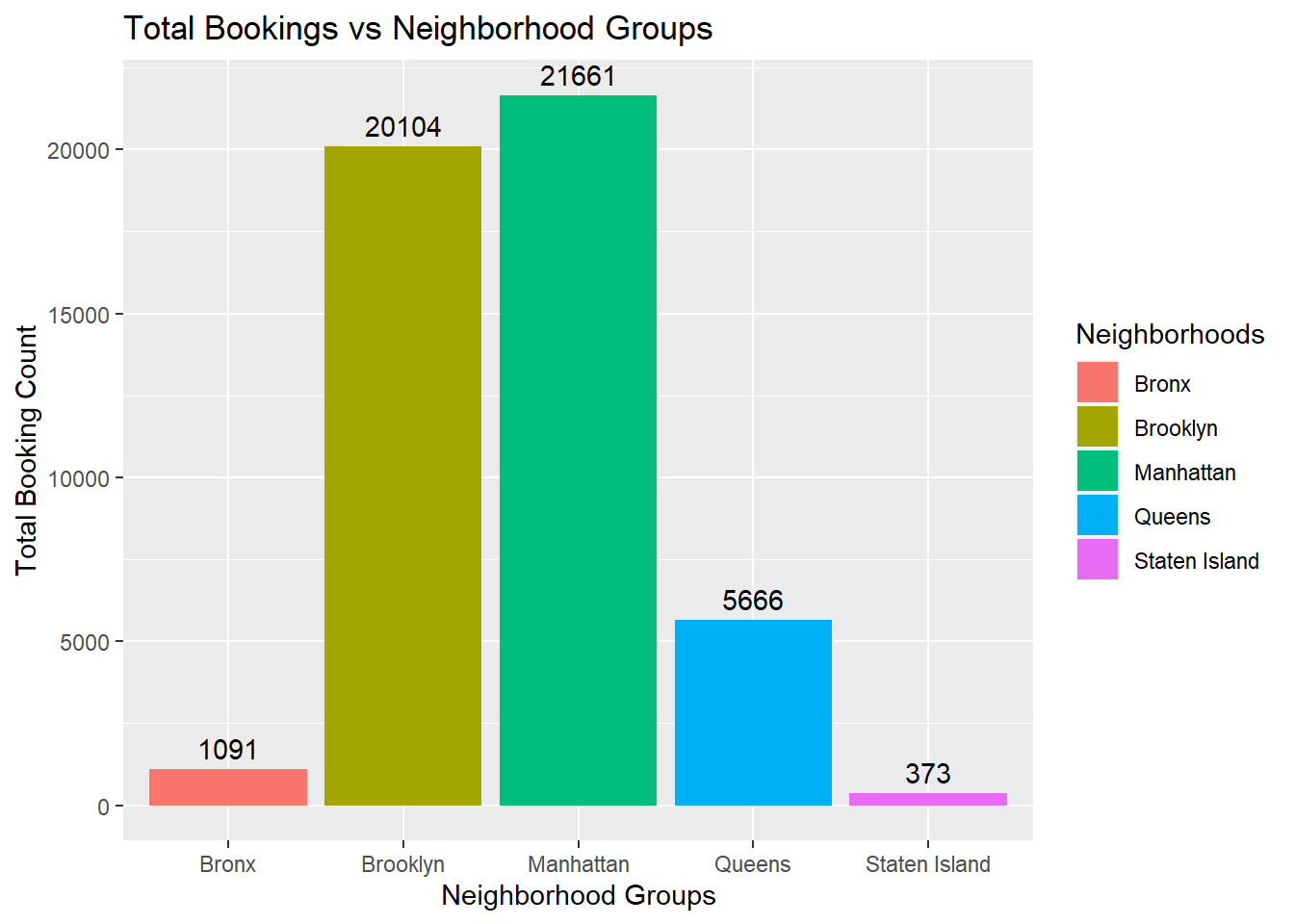
NYC_data %>%
  ggplot(aes(x=price)) +
  geom_histogram() +
  xlim(0, 1500) +
  xlab("Price ($)") +
  ylab("Number of properties") +
  ggtitle("Histogram of property price distribution in dataset")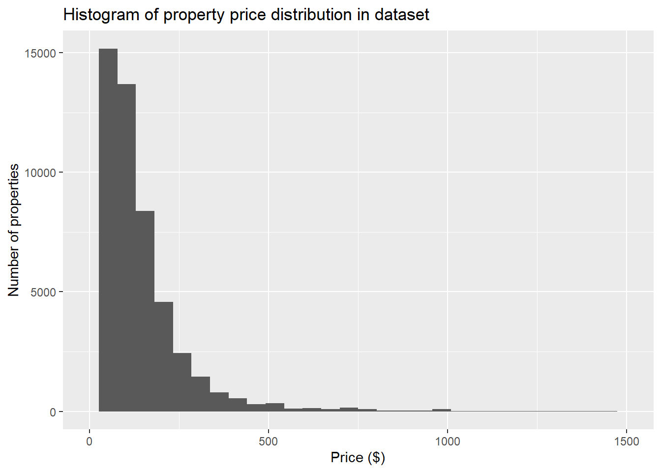
NYC_data %>%
  ggplot(aes(x=minimum_nights)) +
  geom_histogram() +
  xlim(0, 45) +
  xlab("Minimum Nights") +
  ylab("Number of properties") +
  ggtitle("Histogram of minimum nights stayed distribution in dataset")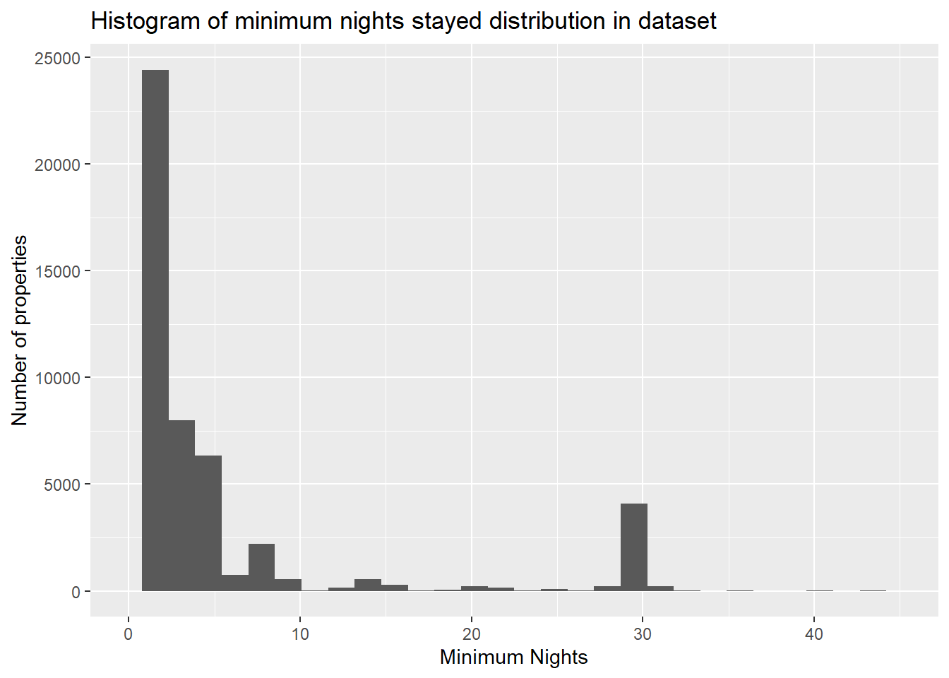
From the visualizations, it can be seen that the most famous neighborhood groups are Manhattan, Brooklyn and then Queens. From the histogram about number of properties vs price, we can see that the price of most properties is less than $500. The second histogram about number of properties vs minimum nights stayed, we can see that mostly people like to stay between 1 to 10 nights, however, quite a large number of guests also book airBNBs for 30 nights.
Bivariate Visualization(s)
ggplot(NYC_data) +
  geom_point(mapping = aes(x = minimum_nights, y = price)) +
  labs(x = "Minimum Nights",
       y = "Price ($)",
       title = "Price vs Minimum Nights Stayed")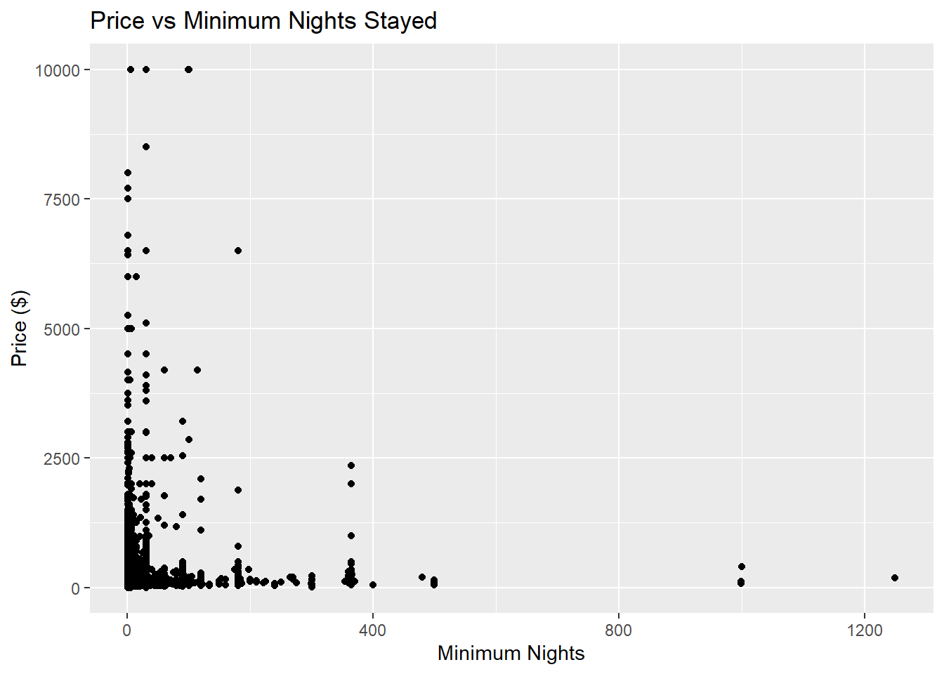
ggplot(NYC_data) +
  geom_bar(aes(x = room_type, fill=neighbourhood_group)) +
  labs(x = "Type of room", y = "Number of Airbnbs", title = "Number of Airbnbs vs  Room Type",
       fill = "Neighbourhood Group")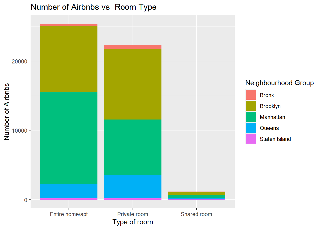
From the bivariate visualizations, we can see the relation between prices and the minimum nights stayed and also the type of rooms that are booked within different neighborhood groups.