library(tidyverse)
library(ggplot2)
library(lubridate)
knitr::opts_chunk$set(echo = TRUE, warning=FALSE, message=FALSE)
Challenge 6 Instructions
challenge_6
hotel_bookings
air_bnb
fed_rate
debt
usa_households
abc_poll
Visualizing Time and Relationships
Challenge Overview
Today’s challenge is to:
- read in a data set, and describe the data set using both words and any supporting information (e.g., tables, etc)
- tidy data (as needed, including sanity checks)
- mutate variables as needed (including sanity checks)
- create at least one graph including time (evolution)
- try to make them “publication” ready (optional)
- Explain why you choose the specific graph type
- Create at least one graph depicting part-whole or flow relationships
- try to make them “publication” ready (optional)
- Explain why you choose the specific graph type
R Graph Gallery is a good starting point for thinking about what information is conveyed in standard graph types, and includes example R code.
(be sure to only include the category tags for the data you use!)
Read in data
Read in one (or more) of the following datasets, using the correct R package and command.
- debt ⭐
- fed_rate ⭐⭐
- abc_poll ⭐⭐⭐
- usa_hh ⭐⭐⭐
- hotel_bookings ⭐⭐⭐⭐
- AB_NYC ⭐⭐⭐⭐⭐
Hotels booking data- (hotel_bookings.csv)
hotel <- read_csv("_data/hotel_bookings.csv", show_col_types = FALSE)
hotel
# A tibble: 119,390 × 32
hotel is_ca…¹ lead_…² arriv…³ arriv…⁴ arriv…⁵ arriv…⁶ stays…⁷ stays…⁸ adults
<chr> <dbl> <dbl> <dbl> <chr> <dbl> <dbl> <dbl> <dbl> <dbl>
1 Resor… 0 342 2015 July 27 1 0 0 2
2 Resor… 0 737 2015 July 27 1 0 0 2
3 Resor… 0 7 2015 July 27 1 0 1 1
4 Resor… 0 13 2015 July 27 1 0 1 1
5 Resor… 0 14 2015 July 27 1 0 2 2
6 Resor… 0 14 2015 July 27 1 0 2 2
7 Resor… 0 0 2015 July 27 1 0 2 2
8 Resor… 0 9 2015 July 27 1 0 2 2
9 Resor… 1 85 2015 July 27 1 0 3 2
10 Resor… 1 75 2015 July 27 1 0 3 2
# … with 119,380 more rows, 22 more variables: children <dbl>, babies <dbl>,
# meal <chr>, country <chr>, market_segment <chr>,
# distribution_channel <chr>, is_repeated_guest <dbl>,
# previous_cancellations <dbl>, previous_bookings_not_canceled <dbl>,
# reserved_room_type <chr>, assigned_room_type <chr>, booking_changes <dbl>,
# deposit_type <chr>, agent <chr>, company <chr>, days_in_waiting_list <dbl>,
# customer_type <chr>, adr <dbl>, required_car_parking_spaces <dbl>, …Briefly describe the data
Tidy Data (as needed)
Is your data already tidy, or is there work to be done? Be sure to anticipate your end result to provide a sanity check, and document your work here.
To count the number of unique values in all the columns we will do,
rapply(hotel,function(x)length(unique(x))) hotel is_canceled
2 2
lead_time arrival_date_year
479 3
arrival_date_month arrival_date_week_number
12 53
arrival_date_day_of_month stays_in_weekend_nights
31 17
stays_in_week_nights adults
35 14
children babies
6 5
meal country
5 178
market_segment distribution_channel
8 5
is_repeated_guest previous_cancellations
2 15
previous_bookings_not_canceled reserved_room_type
73 10
assigned_room_type booking_changes
12 21
deposit_type agent
3 334
company days_in_waiting_list
353 128
customer_type adr
4 8879
required_car_parking_spaces total_of_special_requests
5 6
reservation_status reservation_status_date
3 926 Are there any variables that require mutation to be usable in your analysis stream? For example, do you need to calculate new values in order to graph them? Can string values be represented numerically? Do you need to turn any variables into factors and reorder for ease of graphics and visualization?
Document your work here.
To find the unique values for the hotel we will do,
unique(hotel$hotel)[1] "Resort Hotel" "City Hotel" table(hotel$country)
  ABW   AGO   AIA   ALB   AND   ARE   ARG   ARM   ASM   ATA   ATF   AUS   AUT
    2   362     1    12     7    51   214     8     1     2     1   426  1263
  AZE   BDI   BEL   BEN   BFA   BGD   BGR   BHR   BHS   BIH   BLR   BOL   BRA
   17     1  2342     3     1    12    75     5     1    13    26    10  2224
  BRB   BWA   CAF   CHE   CHL   CHN   CIV   CMR    CN   COL   COM   CPV   CRI
    4     1     5  1730    65   999     6    10  1279    71     2    24    19
  CUB   CYM   CYP   CZE   DEU   DJI   DMA   DNK   DOM   DZA   ECU   EGY   ESP
    8     1    51   171  7287     1     1   435    14   103    27    32  8568
  EST   ETH   FIN   FJI   FRA   FRO   GAB   GBR   GEO   GGY   GHA   GIB   GLP
   83     3   447     1 10415     5     4 12129    22     3     4    18     2
  GNB   GRC   GTM   GUY   HKG   HND   HRV   HUN   IDN   IMN   IND   IRL   IRN
    9   128     4     1    29     1   100   230    35     2   152  3375    83
  IRQ   ISL   ISR   ITA   JAM   JEY   JOR   JPN   KAZ   KEN   KHM   KIR   KNA
   14    57   669  3766     6     8    21   197    19     6     2     1     2
  KOR   KWT   LAO   LBN   LBY   LCA   LIE   LKA   LTU   LUX   LVA   MAC   MAR
  133    16     2    31     8     1     3     7    81   287    55    16   259
  MCO   MDG   MDV   MEX   MKD   MLI   MLT   MMR   MNE   MOZ   MRT   MUS   MWI
    4     1    12    85    10     1    18     1     5    67     1     7     2
  MYS   MYT   NAM   NCL   NGA   NIC   NLD   NOR   NPL  NULL   NZL   OMN   PAK
   28     2     1     1    34     1  2104   607     1   488    74    18    14
  PAN   PER   PHL   PLW   POL   PRI   PRT   PRY   PYF   QAT   ROU   RUS   RWA
    9    29    40     1   919    12 48590     4     1    15   500   632     2
  SAU   SDN   SEN   SGP   SLE   SLV   SMR   SRB   STP   SUR   SVK   SVN   SWE
   48     1    11    39     1     2     1   101     2     5    65    57  1024
  SYC   SYR   TGO   THA   TJK   TMP   TUN   TUR   TWN   TZA   UGA   UKR   UMI
    2     3     2    59     9     3    39   248    51     5     2    68     1
  URY   USA   UZB   VEN   VGB   VNM   ZAF   ZMB   ZWE
32 2097 4 26 1 8 80 2 4 head(hotel)# A tibble: 6 × 32
hotel is_ca…¹ lead_…² arriv…³ arriv…⁴ arriv…⁵ arriv…⁶ stays…⁷ stays…⁸ adults
<chr> <dbl> <dbl> <dbl> <chr> <dbl> <dbl> <dbl> <dbl> <dbl>
1 Resort… 0 342 2015 July 27 1 0 0 2
2 Resort… 0 737 2015 July 27 1 0 0 2
3 Resort… 0 7 2015 July 27 1 0 1 1
4 Resort… 0 13 2015 July 27 1 0 1 1
5 Resort… 0 14 2015 July 27 1 0 2 2
6 Resort… 0 14 2015 July 27 1 0 2 2
# … with 22 more variables: children <dbl>, babies <dbl>, meal <chr>,
# country <chr>, market_segment <chr>, distribution_channel <chr>,
# is_repeated_guest <dbl>, previous_cancellations <dbl>,
# previous_bookings_not_canceled <dbl>, reserved_room_type <chr>,
# assigned_room_type <chr>, booking_changes <dbl>, deposit_type <chr>,
# agent <chr>, company <chr>, days_in_waiting_list <dbl>,
# customer_type <chr>, adr <dbl>, required_car_parking_spaces <dbl>, …lapply(hotel, class)$hotel
[1] "character"
$is_canceled
[1] "numeric"
$lead_time
[1] "numeric"
$arrival_date_year
[1] "numeric"
$arrival_date_month
[1] "character"
$arrival_date_week_number
[1] "numeric"
$arrival_date_day_of_month
[1] "numeric"
$stays_in_weekend_nights
[1] "numeric"
$stays_in_week_nights
[1] "numeric"
$adults
[1] "numeric"
$children
[1] "numeric"
$babies
[1] "numeric"
$meal
[1] "character"
$country
[1] "character"
$market_segment
[1] "character"
$distribution_channel
[1] "character"
$is_repeated_guest
[1] "numeric"
$previous_cancellations
[1] "numeric"
$previous_bookings_not_canceled
[1] "numeric"
$reserved_room_type
[1] "character"
$assigned_room_type
[1] "character"
$booking_changes
[1] "numeric"
$deposit_type
[1] "character"
$agent
[1] "character"
$company
[1] "character"
$days_in_waiting_list
[1] "numeric"
$customer_type
[1] "character"
$adr
[1] "numeric"
$required_car_parking_spaces
[1] "numeric"
$total_of_special_requests
[1] "numeric"
$reservation_status
[1] "character"
$reservation_status_date
[1] "Date"unique(hotel$hotel)[1] "Resort Hotel" "City Hotel" hotelmut <- hotel %>%
mutate(arrival_date = str_c(arrival_date_day_of_month,
arrival_date_month,
arrival_date_year, sep="/"),
arrival_date = dmy(arrival_date),
total_guests = adults + children + babies) %>%
select(-c(arrival_date_day_of_month,arrival_date_month,arrival_date_year))
hotelmut# A tibble: 119,390 × 31
hotel is_ca…¹ lead_…² arriv…³ stays…⁴ stays…⁵ adults child…⁶ babies meal
<chr> <dbl> <dbl> <dbl> <dbl> <dbl> <dbl> <dbl> <dbl> <chr>
1 Resort H… 0 342 27 0 0 2 0 0 BB
2 Resort H… 0 737 27 0 0 2 0 0 BB
3 Resort H… 0 7 27 0 1 1 0 0 BB
4 Resort H… 0 13 27 0 1 1 0 0 BB
5 Resort H… 0 14 27 0 2 2 0 0 BB
6 Resort H… 0 14 27 0 2 2 0 0 BB
7 Resort H… 0 0 27 0 2 2 0 0 BB
8 Resort H… 0 9 27 0 2 2 0 0 FB
9 Resort H… 1 85 27 0 3 2 0 0 BB
10 Resort H… 1 75 27 0 3 2 0 0 HB
# … with 119,380 more rows, 21 more variables: country <chr>,
# market_segment <chr>, distribution_channel <chr>, is_repeated_guest <dbl>,
# previous_cancellations <dbl>, previous_bookings_not_canceled <dbl>,
# reserved_room_type <chr>, assigned_room_type <chr>, booking_changes <dbl>,
# deposit_type <chr>, agent <chr>, company <chr>, days_in_waiting_list <dbl>,
# customer_type <chr>, adr <dbl>, required_car_parking_spaces <dbl>,
# total_of_special_requests <dbl>, reservation_status <chr>, …To change the data type of the agent and company variables from character to numeric.
hotelmut <- hotelmut %>%
  mutate(across(c(agent, company),~ replace(.,str_detect(., "NULL"), NA))) %>% mutate_at(vars(agent, company),as.numeric)
is.numeric(hotelmut$agent)
[1] TRUETime Dependent Visualization
newplot <- hotelmut %>% select(total_guests, arrival_date) %>%
  group_by(arrival_date) %>%
  summarise(net_guests = sum(total_guests, na.rm=TRUE))

newplot
# A tibble: 793 × 2
arrival_date net_guests
<date> <dbl>
1 2015-07-01 225
2 2015-07-02 190
3 2015-07-03 116
4 2015-07-04 181
5 2015-07-05 113
6 2015-07-06 154
7 2015-07-07 114
8 2015-07-08 139
9 2015-07-09 169
10 2015-07-10 120
# … with 783 more rowssummary(newplot$arrival_date) Min. 1st Qu. Median Mean 3rd Qu. Max.
"2015-07-01" "2016-01-15" "2016-07-31" "2016-07-31" "2017-02-14" "2017-08-31" newplot1 <- ggplot(newplot, aes(x = arrival_date, y = net_guests)) +
ggtitle("Guest Count Vs. Arrival Date Trend: Jul 2015 - Jun 2016") +
geom_line(color = "darkgreen") +
xlab("") +
theme(axis.text.x = element_text(angle = 60, hjust = 1, colour = "red"),
axis.text.y = element_text(colour = "red"),
plot.background = element_rect(fill = "lightblue"),
text = element_text(family = "Courier New")) +
scale_x_date(date_labels = "%Y %b %d", date_minor_breaks = "1 month",
limit = c(as.Date("2015-07-01"), as.Date("2016-07-01")))
newplot1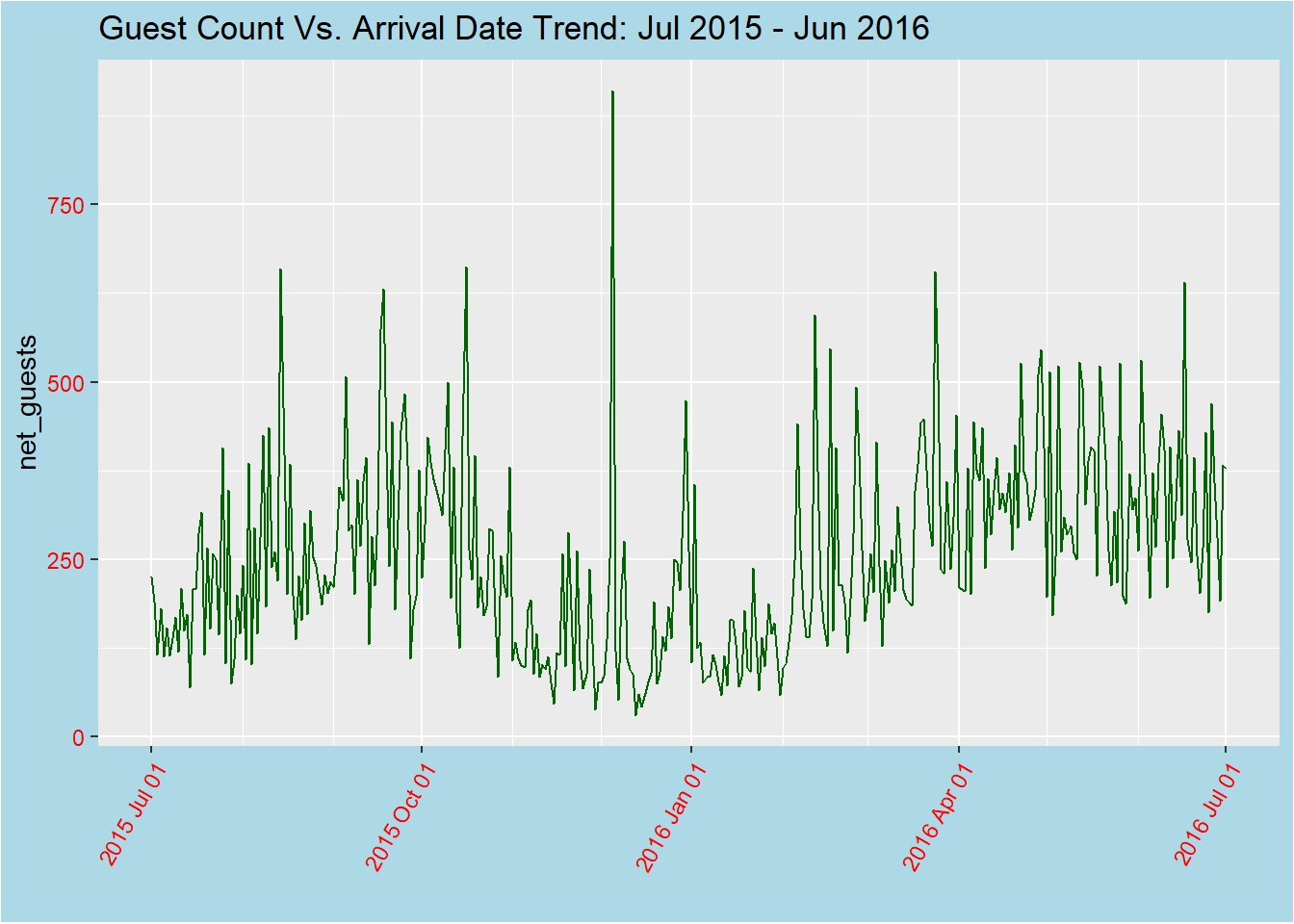
data in the newplot data frame, with the x-axis showing the arrival_date variable and the y-axis showing the net_guests variable. The plot has a title, Guest Count Vs. Arrival Date Trend: Jul 2015 - Jun 2016, and the line is colored dark green.The x-axis uses custom date labels, shows minor breaks every month, and it is limited to the range of dates from July 1, 2015 to July 1, 2016. So, basically it creates a line graph to visualize trends for one year, from July 2015 to July 2016, using time series data. The graph shows the total number of guests who arrived on each day during this period. It also displays minor breaks for each month. The data reveals that the highest number of guests arrived during the first week of December 2015, followed by a sharp decrease. The number of guests appears to be consistent during the summer months of April, May, and June, which may be due to increased vacation travel during this period.
Visualizing Part-Whole Relationships
# create a bar graph based on deposit_type
library(ggplot2)
ggplot(hotel, aes(deposit_type, fill = hotel)) +
  geom_bar(color = "black", size = 0.5) +
  scale_fill_manual(values = c("#FF0000", "#00FF00", "#0000FF")) +
  theme(panel.background = element_rect(fill = "gray"))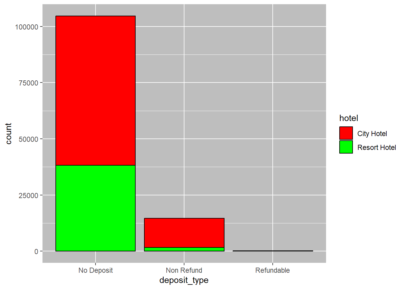
I selected a bar graph with the deposit type on the x-axis because it effectively illustrates the counts of each deposit type by hotel. The graph demonstrates that the majority of bookings from both hotels do not require a deposit. If a deposit is required, the city hotel has a higher number of non-refundable deposits than the resort hotel, which has a small number of refundable deposits. This visual representation clearly shows the differences between the two hotels and the types of deposits they require.
newplot2 <- hotelmut %>%
  filter(reservation_status != 'Canceled', arrival_date >= as.Date("2015-07-01") & arrival_date < as.Date("2016-07-01")) %>%
  select(meal) %>%
  group_by(meal) %>%
  summarise(total_count = n(), .groups = 'drop') %>%
  filter(meal != "Undefined")
newplot2
# A tibble: 4 × 2
meal total_count
<chr> <int>
1 BB 25591
2 FB 210
3 HB 4180
4 SC 1828We uses the filter function to keep only rows that have a reservation_status value other than canceled and an arrival_date within the given date range then it selects only the meal column from the resulting data frame after it groups the data by meal and uses the summarise function to calculate the total count of reservations for each meal plan type. The .groups argument is used to specify that the grouping should be dropped from the output. Finally, the filter function is used again to remove rows with a meal value of Undefined.