Below I have ready in a two week transaction period of cannabis sales at the local dispensary.
On the Read in I have:
Renamed several variables to “delete” as they will not be used in our analysis and thus ignored:
Product Sku: Not necessary because it is replicated with the product name which carries more information
BioTrackId, BioTrack Response, RxNum: These are all categories unused by the business, and do not contain useful information
Remaining Qty: Does not contain any accurate information
Inventory Transactions
#Read in Excel Datatransactions_9_22_2022_10_20_2022_orig <-read_excel("Inventory Transactions 9_22_2022-10_20_2022.xlsx", skip =5,col_names =c("pos_id","product","delete","patient_name","transaction_date","qty_sold","daily_allottment_oz","weight_grams","cost","price","owner_name","owner_location","vendor","sold_by","receipt_no","delete","delete","delete","delete","delete"))%>%select(!contains("delete"))
The transactions data frame we are working with consists of the completed sales transaction at Resinate, Northampton Spanning from 9/22/2022 through 10/05/2022. There are 5,591 instances of 13 variables, meaning that nearly 5,600 transactions were completed during this time period. The variables describe the product type, category, date, patient name, receipt number, budtender, and other transaction information.
Column Mutations
Here I am mutating several variables:
date: I am separating out this date column into hour, minute, and second in order to pin point time of day in which customers are ordering certain products
category, category_names: I created these two variables from the 3 letter abbreviation at the beginning of the product name
#mutating date field and formatting as a datetransactions_9_22_2022_10_20_2022 <- transactions_9_22_2022_10_20_2022_orig%>%mutate(date =as.Date(transaction_date),hour =hour(transaction_date),minute =minute(transaction_date),second =second(transaction_date))%>%mutate(format_date =format(date, "%m/%d/%Y"),format_hour =paste(hour, minute, second, sep =":") )%>%#pulling the category abbreviation to determine category and create a category columnmutate(category =substr(product,1,3) )%>%mutate(category_names =case_when( category =="FLO"| category =="Flo"~"Flower", category =="PRJ"~"Joint", category =="EDI"~"Edible", category =="MIP"~"Marijuana Infused Product", category =="CON"| category =="Con"~"Concentrate", category =="VAP"| category =="Vap"~"Vaporizer", category =="ACC"| category =="Pax"| category =="PAX"| category =="Hig"| category =="Bov"~"Accessories", category =="CLO"| category =="Res"~"Clothing", category =="HTC"~"HTCC Promotion", category =="SAM"~"Samples", category =="TOP"~"Topical", category =="REW"~"Rewards") )
Tidy Data (Sanity Checks)
#ensuring that the category, and category names columns contain no NA values and are accurately codedunique(transactions_9_22_2022_10_20_2022$category_names)
Generated by summarytools 1.0.1 (R version 4.2.1) 2022-11-16
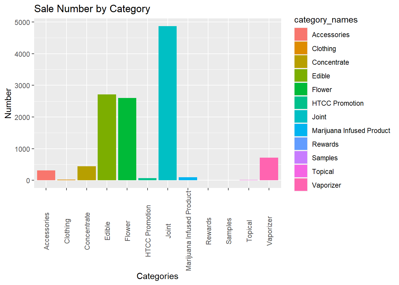
In this farily simple univariate visualization, we can see the number of sales by category. It is clear that Joints are the most popular category followed by Edibles and Flower. This is to be expected in a dispensary as Joints and Edibles are some of the most convenient ways to consume cannabis, followed by Flower that can be ground up and used however the customer pleases.
#univariate visualization of the categoriesggplot(data = transactions_9_22_2022_10_20_2022, mapping =aes(category_names, fill = category_names), size =1) +geom_bar() +ylim(0, NA) +theme(axis.text.x =element_text(angle =90, vjust =0.5)) +ylab("Number") +xlab("Categories")+ggtitle("Sale Number by Category")
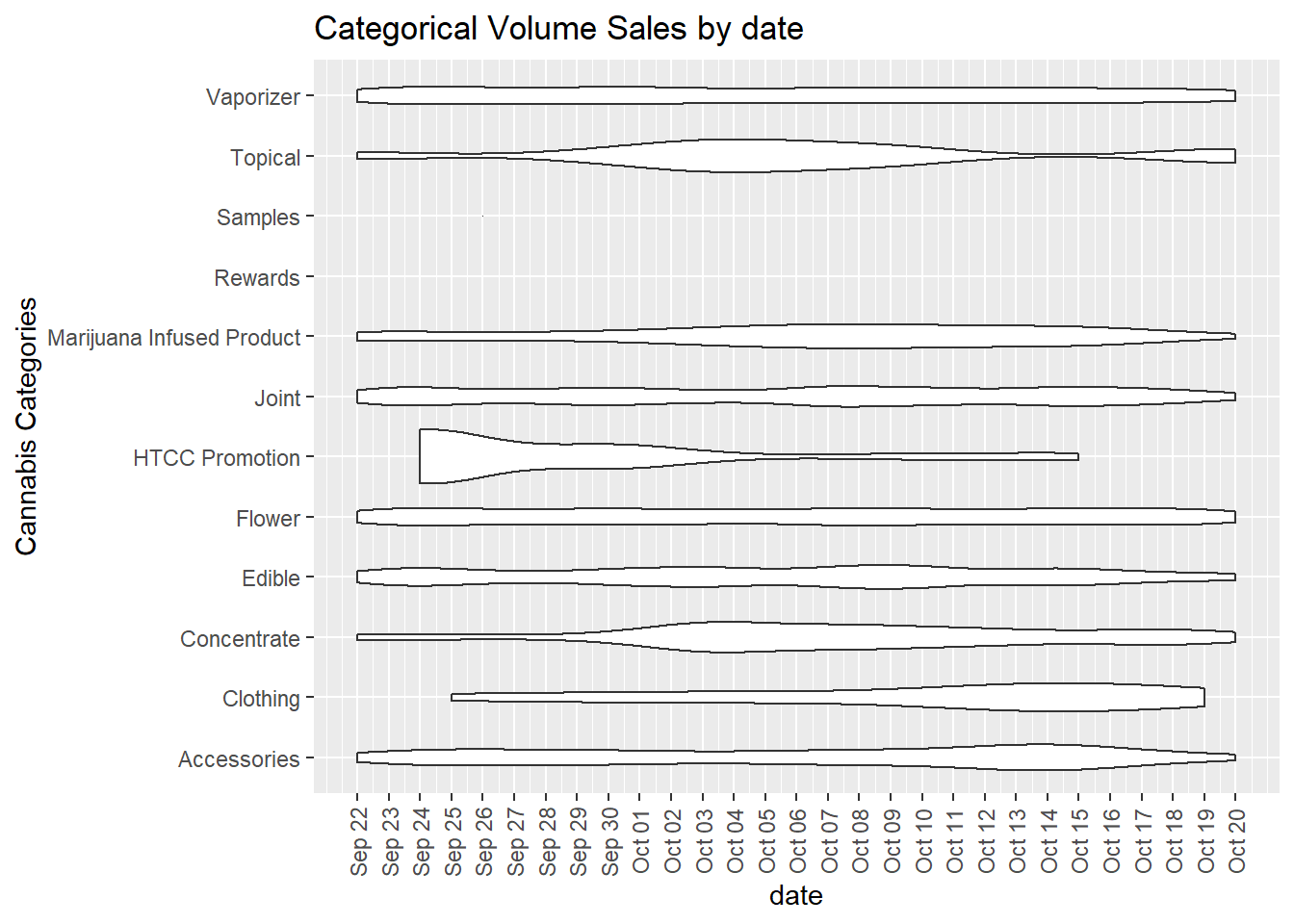
In our first Bivariate visualization we can see the volume of sales by category over time with a violin graph. The volume graph gives a visual representation of popularity of category over time. This can tell us popularity trends, or interest trends by category as well.
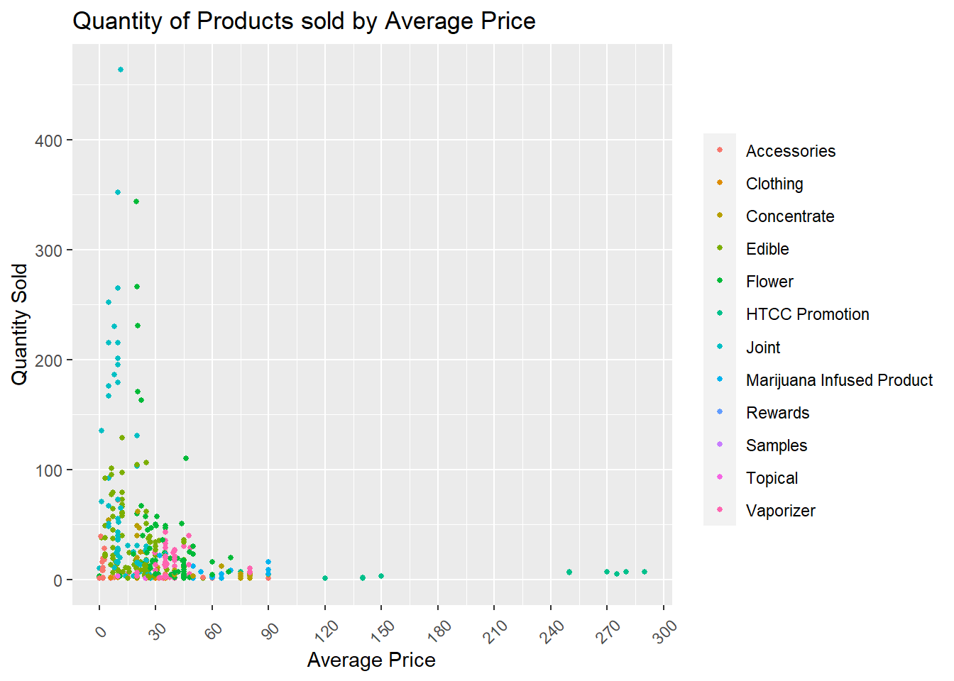
In this second Bivariate Visualization I chose a scatterplot to compare the Average price by product to the quantity sold. I was able to gain the following inside:
Most products are priced between $0 and $90
Within a two week period we are selling approximately 50 units of our most popular products within that price range
We can also see that Joints are the most popular category, with nearly 300 units sold within the given time period.
#creating a flower transactions dataframesold_by_price <- transactions_9_22_2022_10_20_2022%>%group_by(product)%>%mutate(avg_price =mean(price),products_sold =sum(qty_sold))%>%select(-qty_sold)%>%distinct()%>%ggplot(aes(x = avg_price, y = products_sold, color = category_names)) +ylim(0,NA) +scale_x_continuous(breaks =c(0,30,60,90,120,150,180,210,240,270,300)) +geom_point(size =1)+labs(title ="Quantity of Products sold by Average Price")+xlab("Average Price") +ylab("Quantity Sold") +theme(legend.title=element_blank(),axis.text.x =element_text(angle =45, vjust =0.5) )sold_by_price
Source Code
---title: "Challenge 5"author: "Michaela Bowen"description: "Introduction to Visualization"date: "10/19/2022"format: html: toc: true code-copy: true code-tools: truecategories: - challenge_5 - Work Data---```{r}#| label: setup#| warning: false#| message: falselibrary(tidyverse)library(ggplot2)library(readxl)library(lubridate)library(scales)knitr::opts_chunk$set(echo =TRUE, warning=FALSE, message=FALSE)```## Challenge OverviewIn today's Challenge I've attempted to:1) read in a data set, and describe the data set using both words and any supporting information (e.g., tables, etc)2) tidy data (as needed, including sanity checks)3) mutate variables as needed (including sanity checks)4) create at least two univariate visualizations5) Create at least one bivariate visualization::: {.panel-tabset}## Read in and tidy dataBelow I have ready in a two week transaction period of cannabis sales at the local dispensary. On the Read in I have: - Renamed several variables to "delete" as they will not be used in our analysis and thus ignored:+ `Product Sku`: Not necessary because it is replicated with the product name which carries more information + `BioTrackId`, `BioTrack Response`, `RxNum`: These are all categories unused by the business, and do not contain useful information+ `Remaining Qty`: Does not contain *any* accurate information### Inventory Transactions```{r}#| label: read_in#| warning: false#| message: false#Read in Excel Datatransactions_9_22_2022_10_20_2022_orig <-read_excel("Inventory Transactions 9_22_2022-10_20_2022.xlsx", skip =5,col_names =c("pos_id","product","delete","patient_name","transaction_date","qty_sold","daily_allottment_oz","weight_grams","cost","price","owner_name","owner_location","vendor","sold_by","receipt_no","delete","delete","delete","delete","delete"))%>%select(!contains("delete"))```## Briefly describe the dataThe transactions data frame we are working with consists of the completed sales transaction at Resinate, Northampton Spanning from 9/22/2022 through 10/05/2022. There are 5,591 instances of 13 variables, meaning that nearly 5,600 transactions were completed during this time period. The variables describe the product type, category, date, patient name, receipt number, budtender, and other transaction information. ### Column MutationsHere I am mutating several variables:- `date`: I am separating out this date column into hour, minute, and second in order to pin point time of day in which customers are ordering certain products- `category`, `category_names`: I created these two variables from the 3 letter abbreviation at the beginning of the product name```{r}#| label: mutation#| warning: false#| message: false#mutating date field and formatting as a datetransactions_9_22_2022_10_20_2022 <- transactions_9_22_2022_10_20_2022_orig%>%mutate(date =as.Date(transaction_date),hour =hour(transaction_date),minute =minute(transaction_date),second =second(transaction_date))%>%mutate(format_date =format(date, "%m/%d/%Y"),format_hour =paste(hour, minute, second, sep =":") )%>%#pulling the category abbreviation to determine category and create a category columnmutate(category =substr(product,1,3) )%>%mutate(category_names =case_when( category =="FLO"| category =="Flo"~"Flower", category =="PRJ"~"Joint", category =="EDI"~"Edible", category =="MIP"~"Marijuana Infused Product", category =="CON"| category =="Con"~"Concentrate", category =="VAP"| category =="Vap"~"Vaporizer", category =="ACC"| category =="Pax"| category =="PAX"| category =="Hig"| category =="Bov"~"Accessories", category =="CLO"| category =="Res"~"Clothing", category =="HTC"~"HTCC Promotion", category =="SAM"~"Samples", category =="TOP"~"Topical", category =="REW"~"Rewards") )```### Tidy Data (Sanity Checks)```{r}#ensuring that the category, and category names columns contain no NA values and are accurately codedunique(transactions_9_22_2022_10_20_2022$category_names)unique(transactions_9_22_2022_10_20_2022$category)```### Data Summary```{r}#| label: Data Summary#| warning: false#| message: falseprint(summarytools::dfSummary(transactions_9_22_2022_10_20_2022,varnumbers =FALSE,plain.ascii =FALSE, style ="grid", graph.magnif =0.70, valid.col =FALSE),method ='render',table.classes ='table-condensed')```## Univariate VisualizationsIn this farily simple univariate visualization, we can see the number of sales by category. It is clear that Joints are the most popular category followed by Edibles and Flower. This is to be expected in a dispensary as Joints and Edibles are some of the most convenient ways to consume cannabis, followed by Flower that can be ground up and used however the customer pleases.```{r}#| label: Sales by Categorie Univariate#| warning: false#| message: false#univariate visualization of the categoriesggplot(data = transactions_9_22_2022_10_20_2022, mapping =aes(category_names, fill = category_names), size =1) +geom_bar() +ylim(0, NA) +theme(axis.text.x =element_text(angle =90, vjust =0.5)) +ylab("Number") +xlab("Categories")+ggtitle("Sale Number by Category")```## Bivariate Visualization(s)In our first Bivariate visualization we can see the volume of sales by category over time with a violin graph. The volume graph gives a visual representation of popularity of category over time. This can tell us popularity trends, or interest trends by category as well.```{r}#| label: Volume Sales by Date#| warning: false#| message: falseggplot(data = transactions_9_22_2022_10_20_2022, mapping =aes(x = date, y = category_names), size =1) +geom_violin() +theme(legend.title=element_blank(),axis.text.x =element_text(angle =90, vjust =0.5)) +ylab("Cannabis Categories") +scale_x_date(date_labels="%b %d", breaks =unique(transactions_9_22_2022_10_20_2022$date)) +ggtitle("Categorical Volume Sales by date")```In this second Bivariate Visualization I chose a scatterplot to compare the Average price by product to the quantity sold. I was able to gain the following inside:- Most products are priced between $0 and $90 - Within a two week period we are selling approximately 50 units of our most popular products within that price range- We can also see that Joints are the most popular category, with nearly 300 units sold within the given time period. ```{r}#| label: Average Price by Quantity Sold#| warning: false#| message: false#creating a flower transactions dataframesold_by_price <- transactions_9_22_2022_10_20_2022%>%group_by(product)%>%mutate(avg_price =mean(price),products_sold =sum(qty_sold))%>%select(-qty_sold)%>%distinct()%>%ggplot(aes(x = avg_price, y = products_sold, color = category_names)) +ylim(0,NA) +scale_x_continuous(breaks =c(0,30,60,90,120,150,180,210,240,270,300)) +geom_point(size =1)+labs(title ="Quantity of Products sold by Average Price")+xlab("Average Price") +ylab("Quantity Sold") +theme(legend.title=element_blank(),axis.text.x =element_text(angle =45, vjust =0.5) )sold_by_price ```:::