library(tidyverse)
library(ggplot2)
library(readxl)
library(lubridate)
library(scales)
library(viridis)

knitr::opts_chunk$set(echo = TRUE, warning=FALSE, message=FALSE)
Challenge 6
challenge_6
Inventory Transactions 9/22/22-10/20/22
Visualizing Time and Relationships
Challenge Overview
Today’s challenge is to:
- read in a data set, and describe the data set using both words and any supporting information (e.g., tables, etc)
- tidy data (as needed, including sanity checks)
- mutate variables as needed (including sanity checks)
- create at least one graph including time (evolution)
- try to make them “publication” ready (optional)
- Explain why you choose the specific graph type
- Create at least one graph depicting part-whole or flow relationships
- try to make them “publication” ready (optional)
- Explain why you choose the specific graph type
transactions_9_22_2022_10_20_2022_orig <- read_excel("Inventory Transactions 9_22_2022-10_20_2022.xlsx",
    skip = 5,
    col_names = c("pos_id","product","delete","patient_name","transaction_date","qty_sold","daily_allottment_oz","weight_grams","cost","price","owner_name","owner_location","vendor","sold_by","receipt_no","delete","delete","delete","delete","delete"))%>%
  filter(sold_by != "Michaela Bowen")%>%
  select(!contains("delete"))
Briefly describe the data
The transactions data frame we are working with consists of the completed sales transaction at Resinate, Northampton Spanning from 9/22/2022 through 10/20/2022. There are 11,870 instances of 14 variables, meaning that nearly 12,000 items were sold during this time period, between nearly 3,600 transactions.Each instance is a product sold, rather than a complete transaction. All products were sold by 7 employees during this time. The variables describe the product type, category, date, patient name, receipt number, budtender, and other transaction information.
#number of products sold
nrow(transactions_9_22_2022_10_20_2022_orig)
[1] 11802#number of transactions
n_distinct(transactions_9_22_2022_10_20_2022_orig$receipt_no)[1] 3566#number of employees
n_distinct(transactions_9_22_2022_10_20_2022_orig$sold_by)[1] 7#number of customers
n_distinct(transactions_9_22_2022_10_20_2022_orig$patient_name)[1] 2563Here I will mutate columns to better suit the analysis of this data set.
I created 5 intervals that outline the timeframe that I am working with
The columns I plant to mutate:
date: I am separating out this date column into hour, minute, and second in order to pin point time of day in which customers are ordering certain productscategory,category_names: I created these two variables from the 3 letter abbreviation at the beginning of the product name. This will aid in isolating specific categories of product rather thantier: I am planning to create an ordinal column that has the Flower Tier Specification. A,B,C, and D describe the percentage of Total Active Canabinoids in each and thus determine their price.FirstName,LastName: I also separated the first and last name of the Budtender so that I could only include first names in the visualizationweek: After creating the intervals, I used a case when to determine if each date was within said interval and then assigned it week 1-5
transactions_sept22_oct20_working <- transactions_9_22_2022_10_20_2022_orig%>%
#separating date, month, year, minute and second (thinking about removing second option, as it may not be useful)
  mutate(
    date = as.Date(transaction_date),
    day = day(transaction_date),
    hour = hour(transaction_date),
    minute = minute(transaction_date),
    second = second(transaction_date))%>%
  mutate(
    format_date = format(date, "%m/%d/%Y"),
    format_hour = paste(hour, minute, second, sep = ":")
  )%>%
#pulling the category abbreviation to determine category and create a category column
  mutate(
    category = substr(product,1,3)
  )%>%
#changing the abbreviations into full category names
  mutate(
    category_names = case_when(
      category == "FLO" | category == "Flo" ~ "Flower",
      category == "PRJ" ~ "Joint",
      category == "EDI" ~ "Edible",
      category == "MIP" ~ "Marijuana Infused Product",
      category == "CON" | category == "Con" ~ "Concentrate",
      category == "VAP" | category == "Vap" ~ "Vaporizer",
      category == "ACC" | category == "Pax" | category == "PAX" | category == "Hig" | category == "Bov" ~ "Accessories",
      category == "CLO" | category == "Res" ~ "Clothing",
      category == "HTC" ~ "HTCC Promotion",
      category == "SAM" ~ "Samples",
      category == "TOP" ~ "Topical",
      category == "REW" ~ "Rewards")
  )%>%
#created a logical variable to determine if flower was in house, or 3rd party
  mutate(
    house_product = if_else((vendor == "Resinate, Inc."), TRUE, FALSE, NA)
)%>%
  mutate(
   flower_tier = case_when(
     category_names == "Flower" & (price == 48 | price == 50) ~ "A Tier",
     category_names == "Flower" & price == 45 ~ "B Tier",
     category_names == "Flower" & price == 40 ~ "C Tier",
     category_names == "Flower" & (price == 30 | price == 35) ~ "D Tier"
   )
  )%>%
#created an isCannabis boolean column to separate accessories from cannabis product
  mutate(
    isCannabis = case_when(
      category == "FLO"|category == "CON"|category == "VAP"|category == "PRJ"|category == "EDI"|category == "TOP"|category == "HTC"|category == "MIP"|category == "TOP" ~ TRUE,
      category == "ACC" |category == "CLO" | category == "SAM" ~ FALSE
    )
  )%>%
#separating the first and last names of the budtenders for anonymity purposes
  extract(sold_by, c("FirstName", "LastName"), "([^ ]+) (.*)")%>%
#day of the week label
  mutate(weekdayLabel = wday(date, label = TRUE))

#Here I have created my own week intervals rather than the calendar weeks.
week1 <- interval(transactions_sept22_oct20_working$date[1],transactions_sept22_oct20_working$date[1] + days(6))
week2 <- interval(int_end(week1) + days(1), int_end(week1) + days(6))
week3 <- interval(int_end(week2) + days(1), int_end(week2) + days(6))
week4 <- interval(int_end(week3) + days(1), int_end(week3) + days(6))
week5 <- interval(int_end(week4) + days(1), int_end(week4) + days(6))


#here I am categorizing each date by week, and checking if it within the interval i created
transactions_sept22_oct20_working <- transactions_sept22_oct20_working%>%
  mutate(week = case_when(
    date %within% week1 ~ "week 1",
    date %within% week2 ~ "week 2",
    date %within% week3 ~ "week 3",
    date %within% week4 ~ "week 4",
    date %within% week5 ~ "week 5"
  ))
For this time dependent visualization, it is somewhat by time, but because I categorized the dates by week, it may not fit into that category. An additional time dependent visualization would be to have total sales by day over time, however i wanted to see some more information.
To create the Average Sales by Budtender by week, I mutated the following columns:
total_sale_week: Calculating the total sales by each budtender for each weekaverage_sale_week: using a case_when() I calculated the average for each of those
avg_salesby_budtender_by_week <- transactions_sept22_oct20_working%>%
  group_by(week,FirstName)%>%
  mutate(total_sales_week = sum(price))%>%
  mutate(avg_sales_week = case_when(
    week == "week 1" ~ total_sales_week/time_length(week1, "days"),
    week == "week 2" ~ total_sales_week/time_length(week2, "days"),
    week == "week 3" ~ total_sales_week/time_length(week3, "days"),
    week == "week 4" ~ total_sales_week/time_length(week4, "days"),
    week == "week 5" ~ total_sales_week/time_length(week5, "days"),
  ))%>%
  distinct(FirstName, .keep_all = TRUE)%>%
  select(FirstName, week, avg_sales_week)%>%
ggplot(mapping = aes(x = week, y = avg_sales_week, color = FirstName), size = 3,) +
  geom_point() +
  theme(legend.title=element_blank(),axis.text.x = element_text(angle = 45, vjust = 0.5), panel.background = ) +
  ylab("Average Sales ($)") +
  xlab("Weeks 9/22/22 - 10/20/22") +
  ggtitle("Average Sales by Budtender by Week")

avg_salesby_budtender_by_week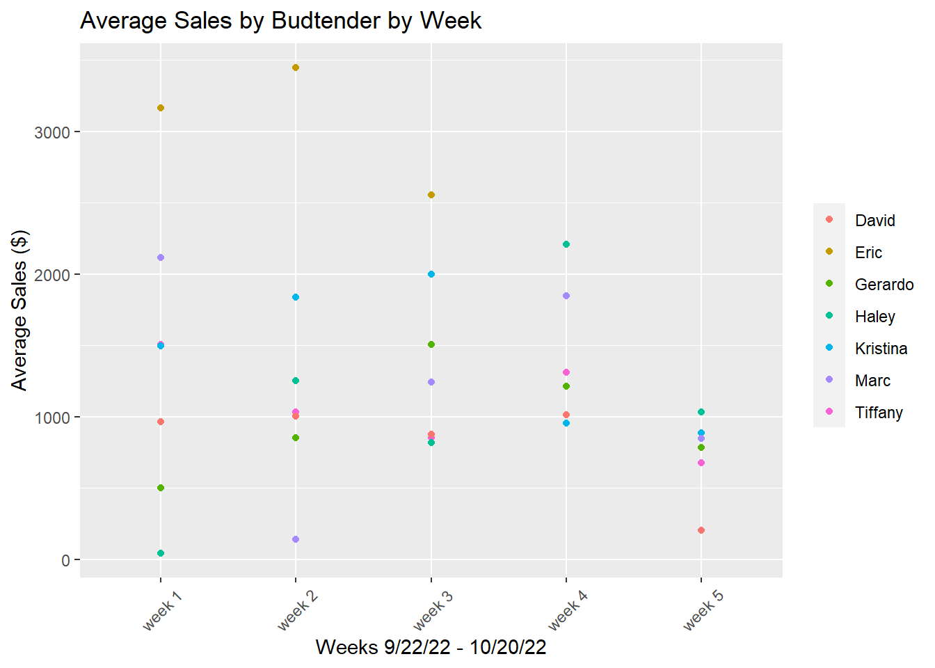
Here my goal was to complete the average sales, by employee, by day of the week. Because my weekday does not start on a sunday, I wanted to figure out a way to count the number of weekdays (how many mondays, tuesdays, wednesdays etc) in the data set. To do this I used n_distinct(week(date)) to determine how many week of the year I was working with. It came p with 5 weeks however, the only day that is present 5 times in this dataset is Thursday.
total_sales_weekday <-transactions_sept22_oct20_working %>%
  group_by(weekdayLabel,FirstName)%>%
  mutate(total_sales = sum(price),
         avg_sales = total_sales/n_distinct(week(date))
  )%>%
  select(weekdayLabel, FirstName,avg_sales, total_sales)%>%
  distinct()%>%
ggplot( mapping = aes(x = weekdayLabel, y = avg_sales, color = FirstName), size = 3,) +
  geom_point() +
  scale_color_viridis(discrete = TRUE, "A") +
  theme(legend.title=element_blank(),axis.text.x = element_text(angle = 45, vjust = 0.5) ) +
  scale_y_continuous(labels = dollar, limits = c(0,5000)) +
  ylab("Average Sales ($)") +
  xlab("Weekday") +
  ggtitle("Average Sales by Budtender by Weekday")

total_sales_weekday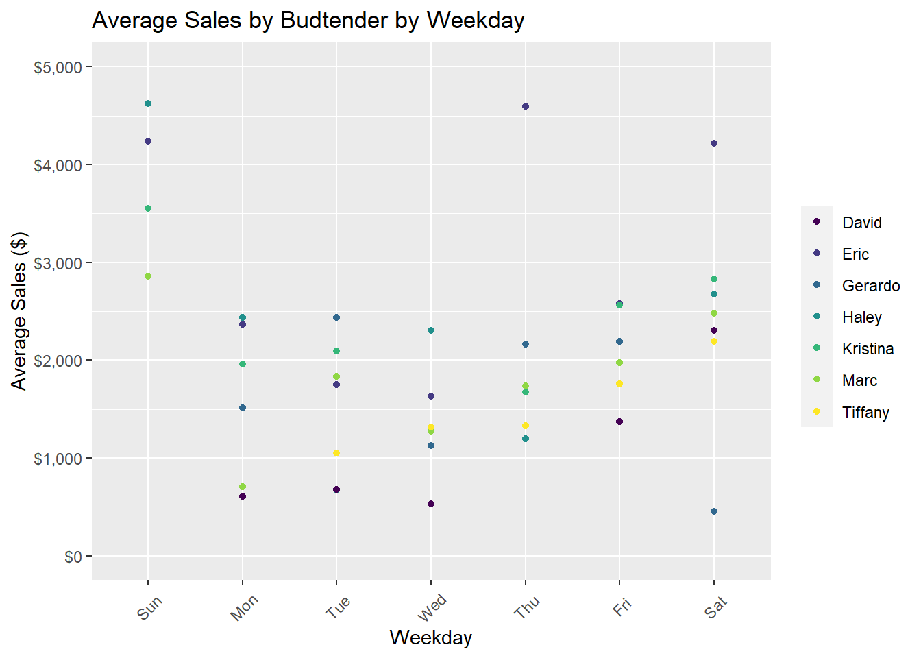
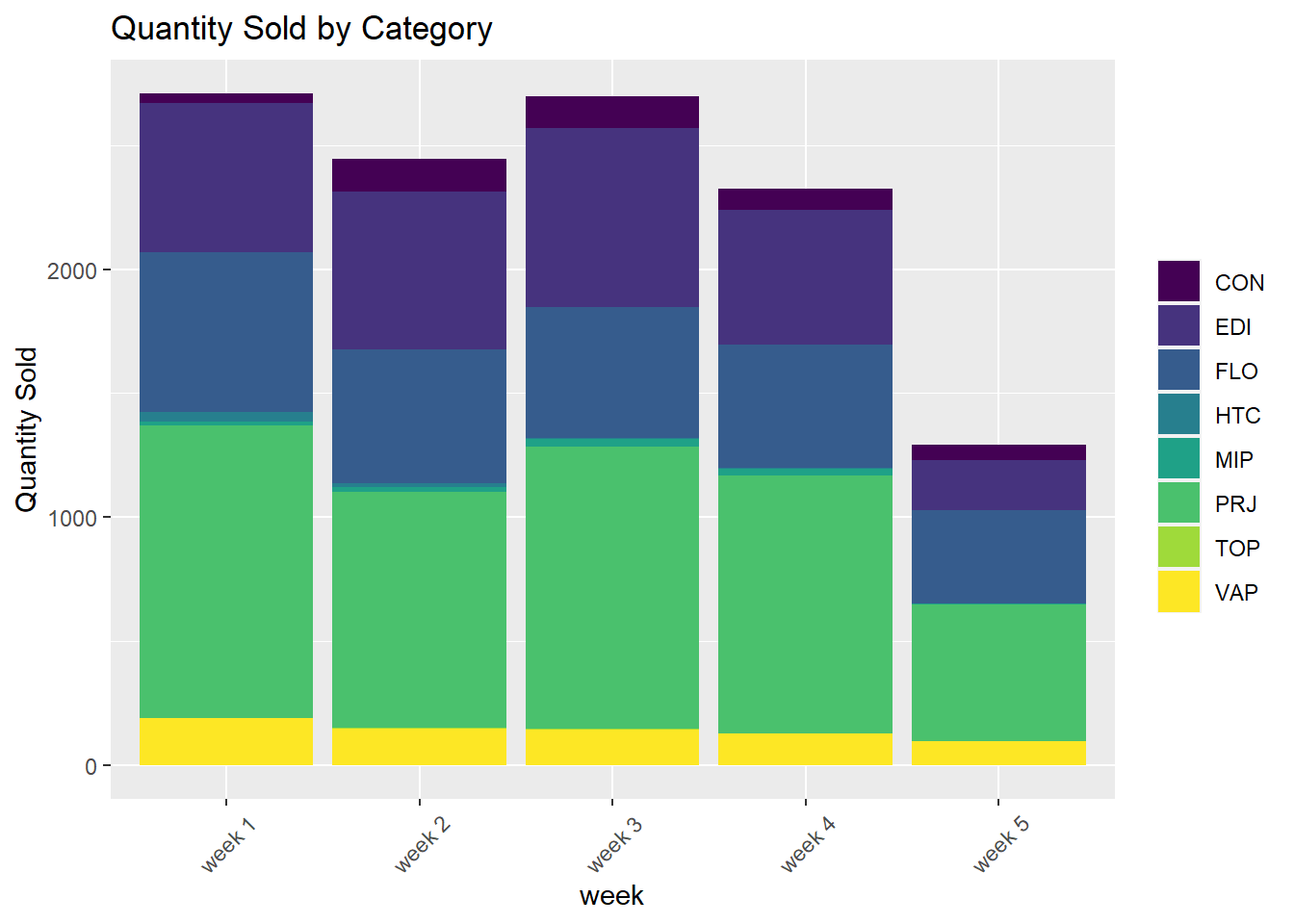
Here I am visualizing total sales by each category of product focusing on Flower, Edibles, Concentrates, and Vapes, Topicals and others which are called Marijuana Infused Products
category_sales <- transactions_sept22_oct20_working%>%
  filter(isCannabis == TRUE)%>%
  group_by(week,category)%>%
  mutate(qty_sold = sum(qty_sold),
         totalSales = sum(price)
         )%>%
  select(week, category, qty_sold, totalSales)%>%
  distinct()%>%
ggplot(mapping = aes(x = week, y = qty_sold, fill = category), size = 3,) +
  geom_col() +
  scale_fill_viridis(discrete = TRUE, "B") +
  theme(legend.title=element_blank(),axis.text.x = element_text(angle = 45, vjust = 0.5) ) +
  ylab("Quantity Sold") +
  ggtitle("Quantity Sold by Category")

category_sales