library(tidyverse)
library(ggplot2)

knitr::opts_chunk$set(echo = TRUE, warning=FALSE, message=FALSE)
Challenge 8
challenge_8
railroads
snl
faostat
debt
Joining Data
Challenge Overview
Today’s challenge is to:
- read in multiple data sets, and describe the data set using both words and any supporting information (e.g., tables, etc)
- tidy data (as needed, including sanity checks)
- mutate variables as needed (including sanity checks)
- join two or more data sets and analyze some aspect of the joined data
(be sure to only include the category tags for the data you use!)
Read in data
Read in one (or more) of the following datasets, using the correct R package and command.
- military marriages ⭐⭐
- faostat ⭐⭐
- railroads ⭐⭐⭐
- fed_rate ⭐⭐⭐
- debt ⭐⭐⭐
- us_hh ⭐⭐⭐⭐
- snl ⭐⭐⭐⭐⭐
country_dataset <- read_csv("_data/FAOSTAT_country_groups.csv")
cattle_dataset <- read_csv("_data/FAOSTAT_cattle_dairy.csv")
Briefly describe the data
I have chosen 2 different datasets to perform the join operation. I have chosen the FAOSTAT country groups and FAOSTAT cattle diary datasets.
The first dataset is basically a codebook that helps in grouping the different countries so that we dont really have to look at the data at a very granular contry level. My main aim is to join the country group variable in order to perform the analysis of the different groups which are within the cattle and dairy dataset.
The second dataset is mainly about the publicly available food and the agriculture data over the 245 countries in the world. It also contains very particular information about the cow milk and also has variables like the units sold and the value of the product. The information from these datasets are from 1960s to 2018. There are 36000+ rows in the dataset.
Tidy Data (as needed)
I have observed that all of the rows have an “area code” which is assigned to the country and I will be using this variable to join the contry group variable. But it is called the “country code” in the country groups file, therefore I am renaming the “area code” variable to be “country code”.
cattle_rename <- rename (cattle_dataset, "Country Code"= "Area Code" )

cattle_rename
# A tibble: 36,449 × 14
Domain Cod…¹ Domain Count…² Area Eleme…³ Element Item …⁴ Item Year …⁵ Year
<chr> <chr> <dbl> <chr> <dbl> <chr> <dbl> <chr> <dbl> <dbl>
1 QL Lives… 2 Afgh… 5318 Milk A… 882 Milk… 1961 1961
2 QL Lives… 2 Afgh… 5420 Yield 882 Milk… 1961 1961
3 QL Lives… 2 Afgh… 5510 Produc… 882 Milk… 1961 1961
4 QL Lives… 2 Afgh… 5318 Milk A… 882 Milk… 1962 1962
5 QL Lives… 2 Afgh… 5420 Yield 882 Milk… 1962 1962
6 QL Lives… 2 Afgh… 5510 Produc… 882 Milk… 1962 1962
7 QL Lives… 2 Afgh… 5318 Milk A… 882 Milk… 1963 1963
8 QL Lives… 2 Afgh… 5420 Yield 882 Milk… 1963 1963
9 QL Lives… 2 Afgh… 5510 Produc… 882 Milk… 1963 1963
10 QL Lives… 2 Afgh… 5318 Milk A… 882 Milk… 1964 1964
# … with 36,439 more rows, 4 more variables: Unit <chr>, Value <dbl>,
# Flag <chr>, `Flag Description` <chr>, and abbreviated variable names
# ¹`Domain Code`, ²`Country Code`, ³`Element Code`, ⁴`Item Code`,
# ⁵`Year Code`Join Data
I am now going to join both of these files using the country code variable.
final <- left_join(cattle_rename, country_dataset, by = "Country Code" )
final
# A tibble: 257,061 × 20
Domain Cod…¹ Domain Count…² Area Eleme…³ Element Item …⁴ Item Year …⁵ Year
<chr> <chr> <dbl> <chr> <dbl> <chr> <dbl> <chr> <dbl> <dbl>
1 QL Lives… 2 Afgh… 5318 Milk A… 882 Milk… 1961 1961
2 QL Lives… 2 Afgh… 5318 Milk A… 882 Milk… 1961 1961
3 QL Lives… 2 Afgh… 5318 Milk A… 882 Milk… 1961 1961
4 QL Lives… 2 Afgh… 5318 Milk A… 882 Milk… 1961 1961
5 QL Lives… 2 Afgh… 5318 Milk A… 882 Milk… 1961 1961
6 QL Lives… 2 Afgh… 5318 Milk A… 882 Milk… 1961 1961
7 QL Lives… 2 Afgh… 5318 Milk A… 882 Milk… 1961 1961
8 QL Lives… 2 Afgh… 5318 Milk A… 882 Milk… 1961 1961
9 QL Lives… 2 Afgh… 5318 Milk A… 882 Milk… 1961 1961
10 QL Lives… 2 Afgh… 5318 Milk A… 882 Milk… 1961 1961
# … with 257,051 more rows, 10 more variables: Unit <chr>, Value <dbl>,
# Flag <chr>, `Flag Description` <chr>, `Country Group Code` <dbl>,
# `Country Group` <chr>, Country <chr>, `M49 Code` <chr>, `ISO2 Code` <chr>,
# `ISO3 Code` <chr>, and abbreviated variable names ¹`Domain Code`,
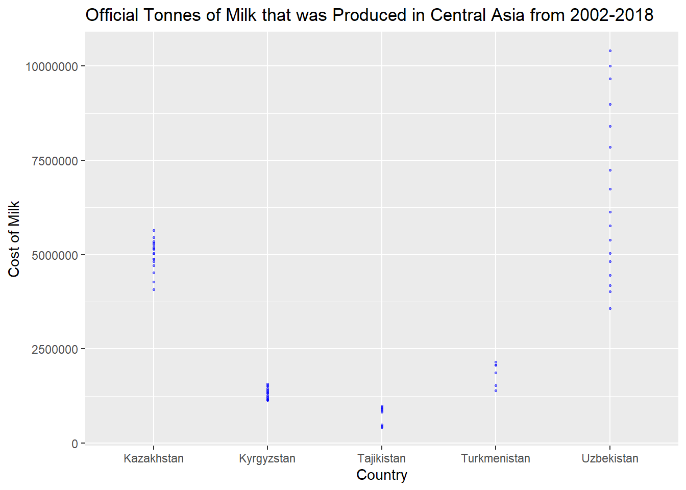
# ²`Country Code`, ³`Element Code`, ⁴`Item Code`, ⁵`Year Code`Now the datasets have been joined and now I want to plot a graph for certain country groups as below.
final %>%
  filter(Year >= 2002) %>%
  filter(`Flag Description` == "Official data") %>%
  filter(`Country Group`=="Central Asia") %>%
  filter(`Unit` == "tonnes") %>%
  ggplot(aes(x=`Area`, y=`Value`)) +
  geom_point(
    color="blue",
    fill="#69b3a2",
    size=.5,
    alpha=.5
  )+
  labs(title = "Official Tonnes of Milk that was Produced in Central Asia from 2002-2018", x="Country", y="Cost of Milk") +
  scale_y_continuous(labels = function(x) format(x, scientific = FALSE))