Challenge 8

Joining Data

library(tidyverse)
library(ggplot2)

knitr::opts_chunk$set(echo = TRUE, warning=FALSE, message=FALSE)

Challenge Overview

Today’s challenge is to:

1. read in multiple data sets, and describe the data set using both words and any supporting information (e.g., tables, etc)
2. tidy data (as needed, including sanity checks)
3. mutate variables as needed (including sanity checks)
4. join two or more data sets and analyze some aspect of the joined data

(be sure to only include the category tags for the data you use!)

Read in data

Using the FAOSTAT dataset

codes <- read_csv("_data/FAOSTAT_country_groups.csv")
cattle <- read_csv("_data/FAOSTAT_cattle_dairy.csv")

Briefly describe the data

The primary dataset I have chosen is the Fao Stat Cattle dataset.It has information about available food and agriculture data from 245 countries. It contains information about cow milk, units sold and price of the product.the data ranges from 1960,s to 2018.

The next file I will using to perform the join is codebook, which groups the data by countries to provide a high level overview, instead of at the country level.

We can then perform join within these datasets and analyze within the country groups.

Tidy Data (as needed)

Matching the column name of the two tables, as one has Area code and one has Country Code. Renaming the cattle Area Code with Country Code.

cattlenew <- rename (cattle, "Country Code"= "Area Code" )
head(cattlenew)

# A tibble: 6 × 14
  Domai…¹ Domain Count…² Area  Eleme…³ Element Item …⁴ Item  Year …⁵  Year Unit 
  <chr>   <chr>    <dbl> <chr>   <dbl> <chr>     <dbl> <chr>   <dbl> <dbl> <chr>
1 QL      Lives…       2 Afgh…    5318 Milk A…     882 Milk…    1961  1961 Head 
2 QL      Lives…       2 Afgh…    5420 Yield       882 Milk…    1961  1961 hg/An
3 QL      Lives…       2 Afgh…    5510 Produc…     882 Milk…    1961  1961 tonn…
4 QL      Lives…       2 Afgh…    5318 Milk A…     882 Milk…    1962  1962 Head 
5 QL      Lives…       2 Afgh…    5420 Yield       882 Milk…    1962  1962 hg/An
6 QL      Lives…       2 Afgh…    5510 Produc…     882 Milk…    1962  1962 tonn…
# … with 3 more variables: Value <dbl>, Flag <chr>, `Flag Description` <chr>,
#   and abbreviated variable names ¹​`Domain Code`, ²​`Country Code`,
#   ³​`Element Code`, ⁴​`Item Code`, ⁵​`Year Code`

Join Data

We can perform left join by using the Country Code

cattlefinal <- left_join(cattlenew, codes, by = "Country Code" )
head(cattlefinal)

# A tibble: 6 × 20
  Domai…¹ Domain Count…² Area  Eleme…³ Element Item …⁴ Item  Year …⁵  Year Unit 
  <chr>   <chr>    <dbl> <chr>   <dbl> <chr>     <dbl> <chr>   <dbl> <dbl> <chr>
1 QL      Lives…       2 Afgh…    5318 Milk A…     882 Milk…    1961  1961 Head 
2 QL      Lives…       2 Afgh…    5318 Milk A…     882 Milk…    1961  1961 Head 
3 QL      Lives…       2 Afgh…    5318 Milk A…     882 Milk…    1961  1961 Head 
4 QL      Lives…       2 Afgh…    5318 Milk A…     882 Milk…    1961  1961 Head 
5 QL      Lives…       2 Afgh…    5318 Milk A…     882 Milk…    1961  1961 Head 
6 QL      Lives…       2 Afgh…    5318 Milk A…     882 Milk…    1961  1961 Head 
# … with 9 more variables: Value <dbl>, Flag <chr>, `Flag Description` <chr>,
#   `Country Group Code` <dbl>, `Country Group` <chr>, Country <chr>,
#   `M49 Code` <chr>, `ISO2 Code` <chr>, `ISO3 Code` <chr>, and abbreviated
#   variable names ¹​`Domain Code`, ²​`Country Code`, ³​`Element Code`,
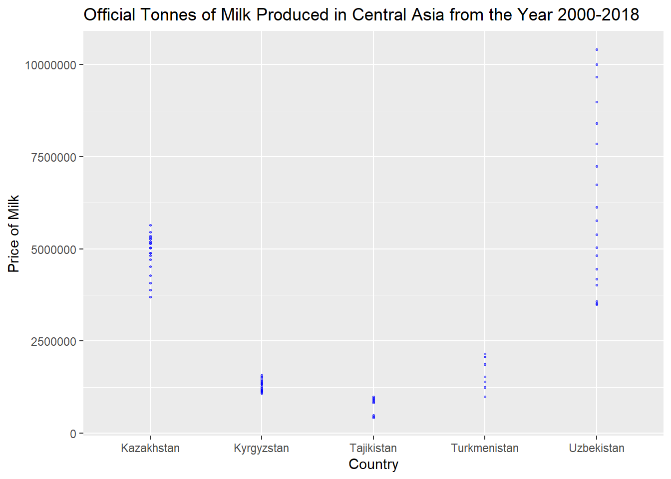
#   ⁴​`Item Code`, ⁵​`Year Code`

After performing join, we can now display the graph by Country Code.

cattlefinal %>%
  filter(Year >= 2000) %>%
  filter(`Flag Description` == "Official data") %>%
  filter(`Country Group`=="Central Asia") %>%
  filter(`Unit` == "tonnes") %>%
  ggplot(aes(x=`Area`, y=`Value`)) + 
  geom_point(
    color="blue",
    fill="#69b3a2",
    size=.5,
    alpha=.5
  )+
  labs(title = "Official Tonnes of Milk Produced in Central Asia from the Year 2000-2018", x="Country", y="Price of Milk") +
  scale_y_continuous(labels = function(x) format(x, scientific = FALSE))