Challenge 8 Instructions

Joining Data

library(tidyverse)
library(ggplot2)
library(readr)
knitr::opts_chunk$set(echo = TRUE, warning=FALSE, message=FALSE)

Challenge Overview

3. mutate variables as needed (including sanity checks)
4. join two or more data sets and analyze some aspect of the joined data

(be sure to only include the category tags for the data you use!)

Read in data

The required data is initially read.

library(readr)
egg_chicken <- read_csv("_data/FAOSTAT_egg_chicken.csv")
cattle_dairy <- read_csv("_data/FAOSTAT_cattle_dairy.csv")
livestock <- read_csv("_data/FAOSTAT_livestock.csv")

Briefly describe the data

While we make efforts to understand the data, we see all the column names present, the sample head of the three datasets.

colnames(egg_chicken)

 [1] "Domain Code"      "Domain"           "Area Code"        "Area"            
 [5] "Element Code"     "Element"          "Item Code"        "Item"            
 [9] "Year Code"        "Year"             "Unit"             "Value"           
[13] "Flag"             "Flag Description"

colnames(cattle_dairy)

 [1] "Domain Code"      "Domain"           "Area Code"        "Area"            
 [5] "Element Code"     "Element"          "Item Code"        "Item"            
 [9] "Year Code"        "Year"             "Unit"             "Value"           
[13] "Flag"             "Flag Description"

colnames(livestock)

 [1] "Domain Code"      "Domain"           "Area Code"        "Area"            
 [5] "Element Code"     "Element"          "Item Code"        "Item"            
 [9] "Year Code"        "Year"             "Unit"             "Value"           
[13] "Flag"             "Flag Description"

head(cattle_dairy)

# A tibble: 6 × 14
  Domai…¹ Domain Area …² Area  Eleme…³ Element Item …⁴ Item  Year …⁵  Year Unit 
  <chr>   <chr>    <dbl> <chr>   <dbl> <chr>     <dbl> <chr>   <dbl> <dbl> <chr>
1 QL      Lives…       2 Afgh…    5318 Milk A…     882 Milk…    1961  1961 Head 
2 QL      Lives…       2 Afgh…    5420 Yield       882 Milk…    1961  1961 hg/An
3 QL      Lives…       2 Afgh…    5510 Produc…     882 Milk…    1961  1961 tonn…
4 QL      Lives…       2 Afgh…    5318 Milk A…     882 Milk…    1962  1962 Head 
5 QL      Lives…       2 Afgh…    5420 Yield       882 Milk…    1962  1962 hg/An
6 QL      Lives…       2 Afgh…    5510 Produc…     882 Milk…    1962  1962 tonn…
# … with 3 more variables: Value <dbl>, Flag <chr>, `Flag Description` <chr>,
#   and abbreviated variable names ¹​`Domain Code`, ²​`Area Code`,
#   ³​`Element Code`, ⁴​`Item Code`, ⁵​`Year Code`

head(egg_chicken)

# A tibble: 6 × 14
  Domai…¹ Domain Area …² Area  Eleme…³ Element Item …⁴ Item  Year …⁵  Year Unit 
  <chr>   <chr>    <dbl> <chr>   <dbl> <chr>     <dbl> <chr>   <dbl> <dbl> <chr>
1 QL      Lives…       2 Afgh…    5313 Laying     1062 Eggs…    1961  1961 1000…
2 QL      Lives…       2 Afgh…    5410 Yield      1062 Eggs…    1961  1961 100m…
3 QL      Lives…       2 Afgh…    5510 Produc…    1062 Eggs…    1961  1961 tonn…
4 QL      Lives…       2 Afgh…    5313 Laying     1062 Eggs…    1962  1962 1000…
5 QL      Lives…       2 Afgh…    5410 Yield      1062 Eggs…    1962  1962 100m…
6 QL      Lives…       2 Afgh…    5510 Produc…    1062 Eggs…    1962  1962 tonn…
# … with 3 more variables: Value <dbl>, Flag <chr>, `Flag Description` <chr>,
#   and abbreviated variable names ¹​`Domain Code`, ²​`Area Code`,
#   ³​`Element Code`, ⁴​`Item Code`, ⁵​`Year Code`

head(livestock)

# A tibble: 6 × 14
  Domai…¹ Domain Area …² Area  Eleme…³ Element Item …⁴ Item  Year …⁵  Year Unit 
  <chr>   <chr>    <dbl> <chr>   <dbl> <chr>     <dbl> <chr>   <dbl> <dbl> <chr>
1 QA      Live …       2 Afgh…    5111 Stocks     1107 Asses    1961  1961 Head 
2 QA      Live …       2 Afgh…    5111 Stocks     1107 Asses    1962  1962 Head 
3 QA      Live …       2 Afgh…    5111 Stocks     1107 Asses    1963  1963 Head 
4 QA      Live …       2 Afgh…    5111 Stocks     1107 Asses    1964  1964 Head 
5 QA      Live …       2 Afgh…    5111 Stocks     1107 Asses    1965  1965 Head 
6 QA      Live …       2 Afgh…    5111 Stocks     1107 Asses    1966  1966 Head 
# … with 3 more variables: Value <dbl>, Flag <chr>, `Flag Description` <chr>,
#   and abbreviated variable names ¹​`Domain Code`, ²​`Area Code`,
#   ³​`Element Code`, ⁴​`Item Code`, ⁵​`Year Code`

table(egg_chicken$Item)

Eggs, hen, in shell 
              38170 

table(cattle_dairy$Item)

Milk, whole fresh cow 
                36449 

table(livestock$Item)

    Asses Buffaloes    Camels    Cattle     Goats    Horses     Mules      Pigs 
     8571      3505      3265     13086     12498     11104      6153     12015 
    Sheep 
    11919 

we observe that only in live stock table we have multiple items.

all(egg_chicken$Year==egg_chicken$`Year Code`)

[1] TRUE

all(cattle_dairy$Year==cattle_dairy$`Year Code`)

[1] TRUE

all(livestock$Year==livestock$`Year Code`)

[1] TRUE

we observe duplicated columns in the data sets.

sapply(egg_chicken,function(x)sum(is.na(x)))

     Domain Code           Domain        Area Code             Area 
               0                0                0                0 
    Element Code          Element        Item Code             Item 
               0                0                0                0 
       Year Code             Year             Unit            Value 
               0                0                0               40 
            Flag Flag Description 
            7548                0 

we see that there are 40 missing values of value and 7548 missing values of flag description.

sapply(cattle_dairy,function(x)sum(is.na(x)))

     Domain Code           Domain        Area Code             Area 
               0                0                0                0 
    Element Code          Element        Item Code             Item 
               0                0                0                0 
       Year Code             Year             Unit            Value 
               0                0                0               74 
            Flag Flag Description 
           10044                0 

sapply(livestock,function(x)sum(is.na(x)))

     Domain Code           Domain        Area Code             Area 
               0                0                0                0 
    Element Code          Element        Item Code             Item 
               0                0                0                0 
       Year Code             Year             Unit            Value 
               0                0                0             1301 
            Flag Flag Description 
           38270                0 

In live_stock there are 1301 missing values in values and 38270 missing values in flags

print(summarytools::dfSummary(egg_chicken,
                        varnumbers = FALSE,
                        plain.ascii  = FALSE, 
                        style        = "grid", 
                        graph.magnif = 0.70, 
                        valid.col    = FALSE),
      method = 'render',
      table.classes = 'table-condensed')

Data Frame Summary

egg_chicken

Dimensions: 38170 x 14
Duplicates: 0

Variable	Stats / Values	Freqs (% of Valid)	Graph	Missing
Domain Code [character]	1. QL	38170 ( 100.0% )		0 (0.0%)
Domain [character]	1. Livestock Primary	38170 ( 100.0% )		0 (0.0%)
Area Code [numeric]	Mean (sd) : 771.1 (1709.6) min ≤ med ≤ max: 1 ≤ 143 ≤ 5504 IQR (CV) : 145 (2.2)	245 distinct values		0 (0.0%)
Area [character]	1. Afghanistan 2. Africa 3. Albania 4. Algeria 5. American Samoa 6. Americas 7. Angola 8. Antigua and Barbuda 9. Argentina 10. Asia [ 235 others ]	174 ( 0.5% ) 174 ( 0.5% ) 174 ( 0.5% ) 174 ( 0.5% ) 174 ( 0.5% ) 174 ( 0.5% ) 174 ( 0.5% ) 174 ( 0.5% ) 174 ( 0.5% ) 174 ( 0.5% ) 36430 ( 95.4% )		0 (0.0%)
Element Code [numeric]	Mean (sd) : 5411.4 (80.5) min ≤ med ≤ max: 5313 ≤ 5410 ≤ 5510 IQR (CV) : 197 (0)	5313 : 12679 ( 33.2% ) 5410 : 12651 ( 33.1% ) 5510 : 12840 ( 33.6% )		0 (0.0%)
Element [character]	1. Laying 2. Production 3. Yield	12679 ( 33.2% ) 12840 ( 33.6% ) 12651 ( 33.1% )		0 (0.0%)
Item Code [numeric]	1 distinct value	1062 : 38170 ( 100.0% )		0 (0.0%)
Item [character]	1. Eggs, hen, in shell	38170 ( 100.0% )		0 (0.0%)
Year Code [numeric]	Mean (sd) : 1990.5 (16.7) min ≤ med ≤ max: 1961 ≤ 1991 ≤ 2018 IQR (CV) : 29 (0)	58 distinct values		0 (0.0%)
Year [numeric]	Mean (sd) : 1990.5 (16.7) min ≤ med ≤ max: 1961 ≤ 1991 ≤ 2018 IQR (CV) : 29 (0)	58 distinct values		0 (0.0%)
Unit [character]	1. 1000 Head 2. 100mg/An 3. tonnes	12679 ( 33.2% ) 12651 ( 33.1% ) 12840 ( 33.6% )		0 (0.0%)
Value [numeric]	Mean (sd) : 291341.2 (2232761) min ≤ med ≤ max: 1 ≤ 31996 ≤ 76769955 IQR (CV) : 91235.8 (7.7)	21325 distinct values		40 (0.1%)
Flag [character]	1. * 2. A 3. F 4. Fc 5. Im 6. M	1435 ( 4.7% ) 3186 ( 10.4% ) 10538 ( 34.4% ) 13344 ( 43.6% ) 2079 ( 6.8% ) 40 ( 0.1% )		7548 (19.8%)
Flag Description [character]	1. Aggregate, may include of 2. Calculated data 3. Data not available 4. FAO data based on imputat 5. FAO estimate 6. Official data 7. Unofficial figure	3186 ( 8.3% ) 13344 ( 35.0% ) 40 ( 0.1% ) 2079 ( 5.4% ) 10538 ( 27.6% ) 7548 ( 19.8% ) 1435 ( 3.8% )		0 (0.0%)

Generated by summarytools 1.0.1 (R version 4.2.1)
2022-12-21

print(summarytools::dfSummary(livestock,
                        varnumbers = FALSE,
                        plain.ascii  = FALSE, 
                        style        = "grid", 
                        graph.magnif = 0.70, 
                        valid.col    = FALSE),
      method = 'render',
      table.classes = 'table-condensed')

Data Frame Summary

livestock

Dimensions: 82116 x 14
Duplicates: 0

Variable	Stats / Values	Freqs (% of Valid)	Graph	Missing
Domain Code [character]	1. QA	82116 ( 100.0% )		0 (0.0%)
Domain [character]	1. Live Animals	82116 ( 100.0% )		0 (0.0%)
Area Code [numeric]	Mean (sd) : 912.7 (1855) min ≤ med ≤ max: 1 ≤ 146 ≤ 5504 IQR (CV) : 148 (2)	253 distinct values		0 (0.0%)
Area [character]	1. Africa 2. Asia 3. China, mainland 4. Eastern Africa 5. Eastern Asia 6. Eastern Europe 7. Egypt 8. Europe 9. India 10. Northern Africa [ 243 others ]	522 ( 0.6% ) 522 ( 0.6% ) 522 ( 0.6% ) 522 ( 0.6% ) 522 ( 0.6% ) 522 ( 0.6% ) 522 ( 0.6% ) 522 ( 0.6% ) 522 ( 0.6% ) 522 ( 0.6% ) 76896 ( 93.6% )		0 (0.0%)
Element Code [numeric]	1 distinct value	5111 : 82116 ( 100.0% )		0 (0.0%)
Element [character]	1. Stocks	82116 ( 100.0% )		0 (0.0%)
Item Code [numeric]	Mean (sd) : 1017.7 (83.3) min ≤ med ≤ max: 866 ≤ 1034 ≤ 1126 IQR (CV) : 120 (0.1)	866 : 13086 ( 15.9% ) 946 : 3505 ( 4.3% ) 976 : 11919 ( 14.5% ) 1016 : 12498 ( 15.2% ) 1034 : 12015 ( 14.6% ) 1096 : 11104 ( 13.5% ) 1107 : 8571 ( 10.4% ) 1110 : 6153 ( 7.5% ) 1126 : 3265 ( 4.0% )		0 (0.0%)
Item [character]	1. Asses 2. Buffaloes 3. Camels 4. Cattle 5. Goats 6. Horses 7. Mules 8. Pigs 9. Sheep	8571 ( 10.4% ) 3505 ( 4.3% ) 3265 ( 4.0% ) 13086 ( 15.9% ) 12498 ( 15.2% ) 11104 ( 13.5% ) 6153 ( 7.5% ) 12015 ( 14.6% ) 11919 ( 14.5% )		0 (0.0%)
Year Code [numeric]	Mean (sd) : 1990.4 (16.8) min ≤ med ≤ max: 1961 ≤ 1991 ≤ 2018 IQR (CV) : 29 (0)	58 distinct values		0 (0.0%)
Year [numeric]	Mean (sd) : 1990.4 (16.8) min ≤ med ≤ max: 1961 ≤ 1991 ≤ 2018 IQR (CV) : 29 (0)	58 distinct values		0 (0.0%)
Unit [character]	1. Head	82116 ( 100.0% )		0 (0.0%)
Value [numeric]	Mean (sd) : 11625569 (64779790) min ≤ med ≤ max: 0 ≤ 224667 ≤ 1489744504 IQR (CV) : 2364200 (5.6)	43667 distinct values		1301 (1.6%)
Flag [character]	1. * 2. A 3. F 4. Im 5. M	2667 ( 6.1% ) 12567 ( 28.7% ) 24550 ( 56.0% ) 2877 ( 6.6% ) 1185 ( 2.7% )		38270 (46.6%)
Flag Description [character]	1. Aggregate, may include of 2. Data not available 3. FAO data based on imputat 4. FAO estimate 5. Official data 6. Unofficial figure	12567 ( 15.3% ) 1185 ( 1.4% ) 2877 ( 3.5% ) 24550 ( 29.9% ) 38270 ( 46.6% ) 2667 ( 3.2% )		0 (0.0%)

Generated by summarytools 1.0.1 (R version 4.2.1)
2022-12-21

print(summarytools::dfSummary(cattle_dairy,
                        varnumbers = FALSE,
                        plain.ascii  = FALSE, 
                        style        = "grid", 
                        graph.magnif = 0.70, 
                        valid.col    = FALSE),
      method = 'render',
      table.classes = 'table-condensed')

Data Frame Summary

cattle_dairy

Dimensions: 36449 x 14
Duplicates: 0

Variable	Stats / Values	Freqs (% of Valid)	Graph	Missing
Domain Code [character]	1. QL	36449 ( 100.0% )		0 (0.0%)
Domain [character]	1. Livestock Primary	36449 ( 100.0% )		0 (0.0%)
Area Code [numeric]	Mean (sd) : 775.2 (1713.8) min ≤ med ≤ max: 1 ≤ 141 ≤ 5504 IQR (CV) : 146 (2.2)	232 distinct values		0 (0.0%)
Area [character]	1. Afghanistan 2. Africa 3. Albania 4. Algeria 5. American Samoa 6. Americas 7. Angola 8. Antigua and Barbuda 9. Argentina 10. Asia [ 222 others ]	174 ( 0.5% ) 174 ( 0.5% ) 174 ( 0.5% ) 174 ( 0.5% ) 174 ( 0.5% ) 174 ( 0.5% ) 174 ( 0.5% ) 174 ( 0.5% ) 174 ( 0.5% ) 174 ( 0.5% ) 34709 ( 95.2% )		0 (0.0%)
Element Code [numeric]	Mean (sd) : 5416 (78.5) min ≤ med ≤ max: 5318 ≤ 5420 ≤ 5510 IQR (CV) : 192 (0)	5318 : 12158 ( 33.4% ) 5420 : 12121 ( 33.3% ) 5510 : 12170 ( 33.4% )		0 (0.0%)
Element [character]	1. Milk Animals 2. Production 3. Yield	12158 ( 33.4% ) 12170 ( 33.4% ) 12121 ( 33.3% )		0 (0.0%)
Item Code [numeric]	1 distinct value	882 : 36449 ( 100.0% )		0 (0.0%)
Item [character]	1. Milk, whole fresh cow	36449 ( 100.0% )		0 (0.0%)
Year Code [numeric]	Mean (sd) : 1990.4 (16.8) min ≤ med ≤ max: 1961 ≤ 1991 ≤ 2018 IQR (CV) : 29 (0)	58 distinct values		0 (0.0%)
Year [numeric]	Mean (sd) : 1990.4 (16.8) min ≤ med ≤ max: 1961 ≤ 1991 ≤ 2018 IQR (CV) : 29 (0)	58 distinct values		0 (0.0%)
Unit [character]	1. Head 2. hg/An 3. tonnes	12158 ( 33.4% ) 12121 ( 33.3% ) 12170 ( 33.4% )		0 (0.0%)
Value [numeric]	Mean (sd) : 4410235 (25744621) min ≤ med ≤ max: 7 ≤ 43266 ≤ 683217055 IQR (CV) : 692151 (5.8)	24088 distinct values		74 (0.2%)
Flag [character]	1. * 2. A 3. F 4. Fc 5. Im 6. M	810 ( 3.1% ) 3070 ( 11.6% ) 7045 ( 26.7% ) 13136 ( 49.7% ) 2270 ( 8.6% ) 74 ( 0.3% )		10044 (27.6%)
Flag Description [character]	1. Aggregate, may include of 2. Calculated data 3. Data not available 4. FAO data based on imputat 5. FAO estimate 6. Official data 7. Unofficial figure	3070 ( 8.4% ) 13136 ( 36.0% ) 74 ( 0.2% ) 2270 ( 6.2% ) 7045 ( 19.3% ) 10044 ( 27.6% ) 810 ( 2.2% )		0 (0.0%)

Generated by summarytools 1.0.1 (R version 4.2.1)
2022-12-21

Tidy the data

First we need to remove the duplicate columns from each of the data set

cattle_diary_new <- subset(cattle_dairy,select= -c(`Year Code`))

head(cattle_diary_new)

# A tibble: 6 × 13
  Domain …¹ Domain Area …² Area  Eleme…³ Element Item …⁴ Item   Year Unit  Value
  <chr>     <chr>    <dbl> <chr>   <dbl> <chr>     <dbl> <chr> <dbl> <chr> <dbl>
1 QL        Lives…       2 Afgh…    5318 Milk A…     882 Milk…  1961 Head  7  e5
2 QL        Lives…       2 Afgh…    5420 Yield       882 Milk…  1961 hg/An 5  e3
3 QL        Lives…       2 Afgh…    5510 Produc…     882 Milk…  1961 tonn… 3.5e5
4 QL        Lives…       2 Afgh…    5318 Milk A…     882 Milk…  1962 Head  7  e5
5 QL        Lives…       2 Afgh…    5420 Yield       882 Milk…  1962 hg/An 5  e3
6 QL        Lives…       2 Afgh…    5510 Produc…     882 Milk…  1962 tonn… 3.5e5
# … with 2 more variables: Flag <chr>, `Flag Description` <chr>, and
#   abbreviated variable names ¹​`Domain Code`, ²​`Area Code`, ³​`Element Code`,
#   ⁴​`Item Code`

livestock_new <- subset(livestock,select= -c(`Year Code`))
egg_new <- subset(egg_chicken,select= -c(`Year Code`))

cattle_diary_new<- cattle_diary_new%>%
  mutate(Item=str_replace_all(Item,"Milk, whole fresh cow", "Milk"))
egg_new <- egg_new%>%
  mutate(Item=str_replace_all(Item,"Eggs, hen, in shell","Poultry"))
table(cattle_diary_mutate$Item)

Error in table(cattle_diary_mutate$Item): object 'cattle_diary_mutate' not found

table(egg_new$Item)

Poultry 
  38170 

Now that we have renamed the columns, now we perform a join on the tidied data.

Join Data

we have same columns in cattle, diary and live stock tables. so when we join them the final data must have the rows summated together in all the tables.

cattle_egg <- full_join(egg_new,cattle_diary_new)
joined_data <- full_join(cattle_egg,livestock_new)

dim(joined_data)

[1] 156735     13

we now confirm that they are all joined together.

Visualizations

ggplot(joined_data,aes(x=Item))+geom_bar(fill = "lightpink") +
  labs(title = "Item and count", x = "Item", 
     y = "Count")+geom_text(stat='count', aes(label=..count..), vjust=1)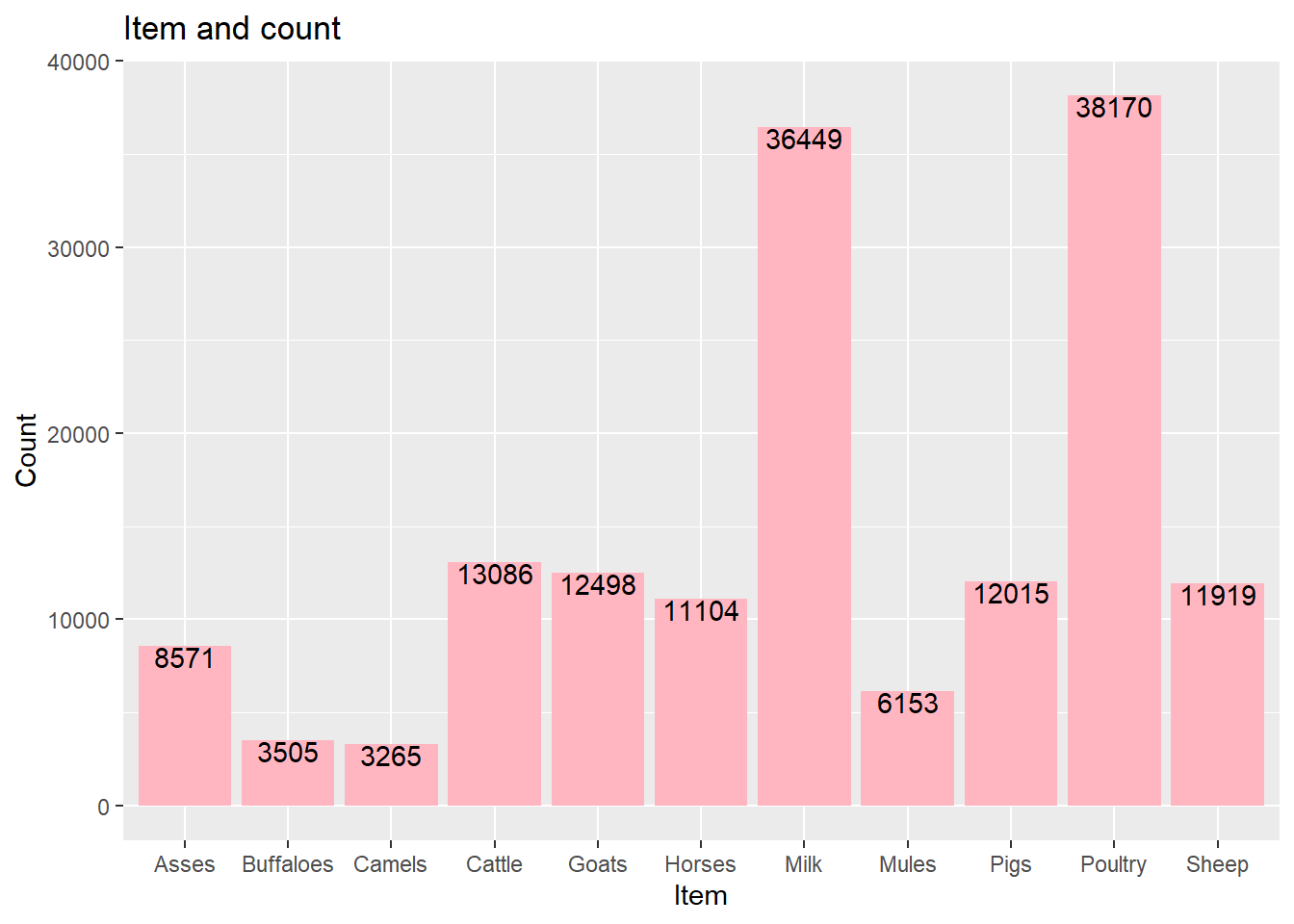

Now, we have understood that we can perform visualizations too on joined data.