library(tidyverse)
library(ggplot2)

knitr::opts_chunk$set(echo = TRUE, warning=FALSE, message=FALSE)
Challenge 6 Solutions
challenge_6
hotel_bookings
air_bnb
fed_rate
debt
usa_households
abc_poll
Visualizing Time and Relationships
Challenge Overview
Today’s challenge is to:
- read in a data set, and describe the data set using both words and any supporting information (e.g., tables, etc)
- tidy data (as needed, including sanity checks)
- mutate variables as needed (including sanity checks)
- create at least one graph including time (evolution)
- try to make them “publication” ready (optional)
- Explain why you choose the specific graph type
- Create at least one graph depicting part-whole or flow relationships
- try to make them “publication” ready (optional)
- Explain why you choose the specific graph type
R Graph Gallery is a good starting point for thinking about what information is conveyed in standard graph types, and includes example R code.
(be sure to only include the category tags for the data you use!)
Read in data
Read in one (or more) of the following datasets, using the correct R package and command.
- debt ⭐
- fed_rate ⭐⭐
- abc_poll ⭐⭐⭐
- usa_hh ⭐⭐⭐
- hotel_bookings ⭐⭐⭐⭐
- AB_NYC ⭐⭐⭐⭐⭐
For this challenge I will be working with the “hotel_bookings” dataset. It is a publicly available data set containing booking transactions from a city hotel and a resort hotel in Portugal.
I used the “hotel_bookings” dataset previously for the Challenge 2 and Challenge 4 and I will be using the same content for the section 1: read in a data set, and describe the data set using both words and any supporting information (e.g., tables, etc), section 2: tidy data (as needed, including sanity checks), and section 3: mutate variables as needed (including sanity checks).
# Reading the hotel_bookings.csv data set and storing in a data frame
hotel_data <- read_csv("_data/hotel_bookings.csv")
print(hotel_data)
# A tibble: 119,390 × 32
hotel is_ca…¹ lead_…² arriv…³ arriv…⁴ arriv…⁵ arriv…⁶ stays…⁷ stays…⁸ adults
<chr> <dbl> <dbl> <dbl> <chr> <dbl> <dbl> <dbl> <dbl> <dbl>
1 Resor… 0 342 2015 July 27 1 0 0 2
2 Resor… 0 737 2015 July 27 1 0 0 2
3 Resor… 0 7 2015 July 27 1 0 1 1
4 Resor… 0 13 2015 July 27 1 0 1 1
5 Resor… 0 14 2015 July 27 1 0 2 2
6 Resor… 0 14 2015 July 27 1 0 2 2
7 Resor… 0 0 2015 July 27 1 0 2 2
8 Resor… 0 9 2015 July 27 1 0 2 2
9 Resor… 1 85 2015 July 27 1 0 3 2
10 Resor… 1 75 2015 July 27 1 0 3 2
# … with 119,380 more rows, 22 more variables: children <dbl>, babies <dbl>,
# meal <chr>, country <chr>, market_segment <chr>,
# distribution_channel <chr>, is_repeated_guest <dbl>,
# previous_cancellations <dbl>, previous_bookings_not_canceled <dbl>,
# reserved_room_type <chr>, assigned_room_type <chr>, booking_changes <dbl>,
# deposit_type <chr>, agent <chr>, company <chr>, days_in_waiting_list <dbl>,
# customer_type <chr>, adr <dbl>, required_car_parking_spaces <dbl>, …Briefly describe the data
#Finding dimension of the data set
dim(hotel_data)
[1] 119390 32#Structure of hotel_data
str(hotel_data)spc_tbl_ [119,390 × 32] (S3: spec_tbl_df/tbl_df/tbl/data.frame)
$ hotel : chr [1:119390] "Resort Hotel" "Resort Hotel" "Resort Hotel" "Resort Hotel" ...
$ is_canceled : num [1:119390] 0 0 0 0 0 0 0 0 1 1 ...
$ lead_time : num [1:119390] 342 737 7 13 14 14 0 9 85 75 ...
$ arrival_date_year : num [1:119390] 2015 2015 2015 2015 2015 ...
$ arrival_date_month : chr [1:119390] "July" "July" "July" "July" ...
$ arrival_date_week_number : num [1:119390] 27 27 27 27 27 27 27 27 27 27 ...
$ arrival_date_day_of_month : num [1:119390] 1 1 1 1 1 1 1 1 1 1 ...
$ stays_in_weekend_nights : num [1:119390] 0 0 0 0 0 0 0 0 0 0 ...
$ stays_in_week_nights : num [1:119390] 0 0 1 1 2 2 2 2 3 3 ...
$ adults : num [1:119390] 2 2 1 1 2 2 2 2 2 2 ...
$ children : num [1:119390] 0 0 0 0 0 0 0 0 0 0 ...
$ babies : num [1:119390] 0 0 0 0 0 0 0 0 0 0 ...
$ meal : chr [1:119390] "BB" "BB" "BB" "BB" ...
$ country : chr [1:119390] "PRT" "PRT" "GBR" "GBR" ...
$ market_segment : chr [1:119390] "Direct" "Direct" "Direct" "Corporate" ...
$ distribution_channel : chr [1:119390] "Direct" "Direct" "Direct" "Corporate" ...
$ is_repeated_guest : num [1:119390] 0 0 0 0 0 0 0 0 0 0 ...
$ previous_cancellations : num [1:119390] 0 0 0 0 0 0 0 0 0 0 ...
$ previous_bookings_not_canceled: num [1:119390] 0 0 0 0 0 0 0 0 0 0 ...
$ reserved_room_type : chr [1:119390] "C" "C" "A" "A" ...
$ assigned_room_type : chr [1:119390] "C" "C" "C" "A" ...
$ booking_changes : num [1:119390] 3 4 0 0 0 0 0 0 0 0 ...
$ deposit_type : chr [1:119390] "No Deposit" "No Deposit" "No Deposit" "No Deposit" ...
$ agent : chr [1:119390] "NULL" "NULL" "NULL" "304" ...
$ company : chr [1:119390] "NULL" "NULL" "NULL" "NULL" ...
$ days_in_waiting_list : num [1:119390] 0 0 0 0 0 0 0 0 0 0 ...
$ customer_type : chr [1:119390] "Transient" "Transient" "Transient" "Transient" ...
$ adr : num [1:119390] 0 0 75 75 98 ...
$ required_car_parking_spaces : num [1:119390] 0 0 0 0 0 0 0 0 0 0 ...
$ total_of_special_requests : num [1:119390] 0 0 0 0 1 1 0 1 1 0 ...
$ reservation_status : chr [1:119390] "Check-Out" "Check-Out" "Check-Out" "Check-Out" ...
$ reservation_status_date : Date[1:119390], format: "2015-07-01" "2015-07-01" ...
- attr(*, "spec")=
.. cols(
.. hotel = col_character(),
.. is_canceled = col_double(),
.. lead_time = col_double(),
.. arrival_date_year = col_double(),
.. arrival_date_month = col_character(),
.. arrival_date_week_number = col_double(),
.. arrival_date_day_of_month = col_double(),
.. stays_in_weekend_nights = col_double(),
.. stays_in_week_nights = col_double(),
.. adults = col_double(),
.. children = col_double(),
.. babies = col_double(),
.. meal = col_character(),
.. country = col_character(),
.. market_segment = col_character(),
.. distribution_channel = col_character(),
.. is_repeated_guest = col_double(),
.. previous_cancellations = col_double(),
.. previous_bookings_not_canceled = col_double(),
.. reserved_room_type = col_character(),
.. assigned_room_type = col_character(),
.. booking_changes = col_double(),
.. deposit_type = col_character(),
.. agent = col_character(),
.. company = col_character(),
.. days_in_waiting_list = col_double(),
.. customer_type = col_character(),
.. adr = col_double(),
.. required_car_parking_spaces = col_double(),
.. total_of_special_requests = col_double(),
.. reservation_status = col_character(),
.. reservation_status_date = col_date(format = "")
.. )
- attr(*, "problems")=<externalptr> #Summary of hotel_data
library(summarytools)
print(summarytools::dfSummary(hotel_data,
varnumbers = FALSE,
plain.ascii = FALSE,
style = "grid",
graph.magnif = 0.60,
valid.col = FALSE),
method = 'render',
table.classes = 'table-condensed')Data Frame Summary
hotel_data
Dimensions: 119390 x 32Duplicates: 31994
| Variable | Stats / Values | Freqs (% of Valid) | Graph | Missing | |||||||||||||||||||||||||||||||||||||||||||||||||||||||
|---|---|---|---|---|---|---|---|---|---|---|---|---|---|---|---|---|---|---|---|---|---|---|---|---|---|---|---|---|---|---|---|---|---|---|---|---|---|---|---|---|---|---|---|---|---|---|---|---|---|---|---|---|---|---|---|---|---|---|---|
| hotel [character] |
|
|
 |
0 (0.0%) | |||||||||||||||||||||||||||||||||||||||||||||||||||||||
| is_canceled [numeric] |
|
|
 |
0 (0.0%) | |||||||||||||||||||||||||||||||||||||||||||||||||||||||
| lead_time [numeric] |
|
479 distinct values |  |
0 (0.0%) | |||||||||||||||||||||||||||||||||||||||||||||||||||||||
| arrival_date_year [numeric] |
|
|
 |
0 (0.0%) | |||||||||||||||||||||||||||||||||||||||||||||||||||||||
| arrival_date_month [character] |
|
|
 |
0 (0.0%) | |||||||||||||||||||||||||||||||||||||||||||||||||||||||
| arrival_date_week_number [numeric] |
|
53 distinct values |  |
0 (0.0%) | |||||||||||||||||||||||||||||||||||||||||||||||||||||||
| arrival_date_day_of_month [numeric] |
|
31 distinct values |  |
0 (0.0%) | |||||||||||||||||||||||||||||||||||||||||||||||||||||||
| stays_in_weekend_nights [numeric] |
|
17 distinct values |  |
0 (0.0%) | |||||||||||||||||||||||||||||||||||||||||||||||||||||||
| stays_in_week_nights [numeric] |
|
35 distinct values |  |
0 (0.0%) | |||||||||||||||||||||||||||||||||||||||||||||||||||||||
| adults [numeric] |
|
14 distinct values |  |
0 (0.0%) | |||||||||||||||||||||||||||||||||||||||||||||||||||||||
| children [numeric] |
|
|
 |
4 (0.0%) | |||||||||||||||||||||||||||||||||||||||||||||||||||||||
| babies [numeric] |
|
|
 |
0 (0.0%) | |||||||||||||||||||||||||||||||||||||||||||||||||||||||
| meal [character] |
|
|
 |
0 (0.0%) | |||||||||||||||||||||||||||||||||||||||||||||||||||||||
| country [character] |
|
|
 |
0 (0.0%) | |||||||||||||||||||||||||||||||||||||||||||||||||||||||
| market_segment [character] |
|
|
 |
0 (0.0%) | |||||||||||||||||||||||||||||||||||||||||||||||||||||||
| distribution_channel [character] |
|
|
 |
0 (0.0%) | |||||||||||||||||||||||||||||||||||||||||||||||||||||||
| is_repeated_guest [numeric] |
|
|
 |
0 (0.0%) | |||||||||||||||||||||||||||||||||||||||||||||||||||||||
| previous_cancellations [numeric] |
|
15 distinct values |  |
0 (0.0%) | |||||||||||||||||||||||||||||||||||||||||||||||||||||||
| previous_bookings_not_canceled [numeric] |
|
73 distinct values |  |
0 (0.0%) | |||||||||||||||||||||||||||||||||||||||||||||||||||||||
| reserved_room_type [character] |
|
|
 |
0 (0.0%) | |||||||||||||||||||||||||||||||||||||||||||||||||||||||
| assigned_room_type [character] |
|
|
 |
0 (0.0%) | |||||||||||||||||||||||||||||||||||||||||||||||||||||||
| booking_changes [numeric] |
|
21 distinct values |  |
0 (0.0%) | |||||||||||||||||||||||||||||||||||||||||||||||||||||||
| deposit_type [character] |
|
|
 |
0 (0.0%) | |||||||||||||||||||||||||||||||||||||||||||||||||||||||
| agent [character] |
|
|
 |
0 (0.0%) | |||||||||||||||||||||||||||||||||||||||||||||||||||||||
| company [character] |
|
|
 |
0 (0.0%) | |||||||||||||||||||||||||||||||||||||||||||||||||||||||
| days_in_waiting_list [numeric] |
|
128 distinct values |  |
0 (0.0%) | |||||||||||||||||||||||||||||||||||||||||||||||||||||||
| customer_type [character] |
|
|
 |
0 (0.0%) | |||||||||||||||||||||||||||||||||||||||||||||||||||||||
| adr [numeric] |
|
8879 distinct values |  |
0 (0.0%) | |||||||||||||||||||||||||||||||||||||||||||||||||||||||
| required_car_parking_spaces [numeric] |
|
|
 |
0 (0.0%) | |||||||||||||||||||||||||||||||||||||||||||||||||||||||
| total_of_special_requests [numeric] |
|
|
 |
0 (0.0%) | |||||||||||||||||||||||||||||||||||||||||||||||||||||||
| reservation_status [character] |
|
|
 |
0 (0.0%) | |||||||||||||||||||||||||||||||||||||||||||||||||||||||
| reservation_status_date [Date] |
|
926 distinct values |  |
0 (0.0%) |
Generated by summarytools 1.0.1 (R version 4.2.1)
2022-12-21
#Check for the period of hotel booking dates
hotel_data%>%
  select(hotel, arrival_date_year, arrival_date_month)%>%distinct()
# A tibble: 52 × 3
hotel arrival_date_year arrival_date_month
<chr> <dbl> <chr>
1 Resort Hotel 2015 July
2 Resort Hotel 2015 August
3 Resort Hotel 2015 September
4 Resort Hotel 2015 October
5 Resort Hotel 2015 November
6 Resort Hotel 2015 December
7 Resort Hotel 2016 January
8 Resort Hotel 2016 February
9 Resort Hotel 2016 March
10 Resort Hotel 2016 April
# … with 42 more rowsAfter reading the data using read_csv function, it is stored in a dataframe “hotel_data”. The hotel_bookings data set contains 119390 rows (observations) and 32 columns (attributes/variables) including information such as when the booking was made, length of stay, the number of adults, children, and/or babies, the number of available parking spaces, and many others for the respective hotels. Each row/observation represents a hotel booking. Since this is a public data set, all data elements pertaining to hotel or customer identification are not included in the data set. This data set can have an important role for research and educational purposes in hotel administration, revenue management, machine learning, data mining and other fields. This data set will be helpful for (i) Tourists (people who are booking hotels) to check and understand trends of hotel price over a period of time and plan their travel accordingly within budget, learn about hotel accommodations and features before booking (ii) Hotel Management to keep track of the relevant information about themselves as well as their competitors. Understand and analyze the seasonal trend of hotel booking and accommodate different types of visitors that they have (iii) Tourist / hospitality services - (e.g. travel agency, airlines / car rental companies) to observe the times when hotels in the region are in high demand, analyze the duration of typical stays, and use the information to help plan their own services (iv) Local Government / independent data analysts to observe the overall trend of tourist activities in the region and analyzing the different types of visitors in the hotels during different seasons.
Using the “dfSummary” function from “summarytools” package we find that there are 31994 duplicates in the data. The reason for the identified duplication is that there is no unique id for each booking. It is possible that the booking was made by different tourists and the values for each attribute was exactly the same. This confusion could have been avoided by adding a Booking ID which would be unique for each booking. 66.4% of the data represents city hotel and the remaining 33.6% of the data represents resort hotel. 18.4%, 47.5% and 34.1% of the data correspondingly represents years 2015, 2016 and 2017. I wanted to check the unequal distribution in data for the 3 consecutive years. I further investigated the data and found that the data we have represents hotel bookings from the period July 2015 - August 2017.
Tidy Data (as needed)
Is your data already tidy, or is there work to be done? Be sure to anticipate your end result to provide a sanity check, and document your work here.
#Check for missing/null data in the hotel_data
sum(is.na(hotel_data))
[1] 4sum(is.null(hotel_data))[1] 0We find that there are 4 NA’s or missing values in the dataset.
# Checking which columns have NA values
col <- colnames(hotel_data)
for (c in col){
  print(paste0("NA values in ", c, ": ", sum(is.na(hotel_data[,c]))))
}
[1] "NA values in hotel: 0"
[1] "NA values in is_canceled: 0"
[1] "NA values in lead_time: 0"
[1] "NA values in arrival_date_year: 0"
[1] "NA values in arrival_date_month: 0"
[1] "NA values in arrival_date_week_number: 0"
[1] "NA values in arrival_date_day_of_month: 0"
[1] "NA values in stays_in_weekend_nights: 0"
[1] "NA values in stays_in_week_nights: 0"
[1] "NA values in adults: 0"
[1] "NA values in children: 4"
[1] "NA values in babies: 0"
[1] "NA values in meal: 0"
[1] "NA values in country: 0"
[1] "NA values in market_segment: 0"
[1] "NA values in distribution_channel: 0"
[1] "NA values in is_repeated_guest: 0"
[1] "NA values in previous_cancellations: 0"
[1] "NA values in previous_bookings_not_canceled: 0"
[1] "NA values in reserved_room_type: 0"
[1] "NA values in assigned_room_type: 0"
[1] "NA values in booking_changes: 0"
[1] "NA values in deposit_type: 0"
[1] "NA values in agent: 0"
[1] "NA values in company: 0"
[1] "NA values in days_in_waiting_list: 0"
[1] "NA values in customer_type: 0"
[1] "NA values in adr: 0"
[1] "NA values in required_car_parking_spaces: 0"
[1] "NA values in total_of_special_requests: 0"
[1] "NA values in reservation_status: 0"
[1] "NA values in reservation_status_date: 0"We can see that all 4 NA’s in the hotel booking dataset are from the column “Children”. We can either replace the missing values with 0 or we can drop the 4 rows with NA values. I chose to drop the 4 rows as removing 4 rows from a huge dataset with 119390 observations/rows would not affect any of the statistics significantly.
# Checking which columns have NULL values
col <- colnames(hotel_data)
for (c in col){
  print(paste0("NULL values in ", c, ": ", sum(is.null(hotel_data[,c]))))
}
[1] "NULL values in hotel: 0"
[1] "NULL values in is_canceled: 0"
[1] "NULL values in lead_time: 0"
[1] "NULL values in arrival_date_year: 0"
[1] "NULL values in arrival_date_month: 0"
[1] "NULL values in arrival_date_week_number: 0"
[1] "NULL values in arrival_date_day_of_month: 0"
[1] "NULL values in stays_in_weekend_nights: 0"
[1] "NULL values in stays_in_week_nights: 0"
[1] "NULL values in adults: 0"
[1] "NULL values in children: 0"
[1] "NULL values in babies: 0"
[1] "NULL values in meal: 0"
[1] "NULL values in country: 0"
[1] "NULL values in market_segment: 0"
[1] "NULL values in distribution_channel: 0"
[1] "NULL values in is_repeated_guest: 0"
[1] "NULL values in previous_cancellations: 0"
[1] "NULL values in previous_bookings_not_canceled: 0"
[1] "NULL values in reserved_room_type: 0"
[1] "NULL values in assigned_room_type: 0"
[1] "NULL values in booking_changes: 0"
[1] "NULL values in deposit_type: 0"
[1] "NULL values in agent: 0"
[1] "NULL values in company: 0"
[1] "NULL values in days_in_waiting_list: 0"
[1] "NULL values in customer_type: 0"
[1] "NULL values in adr: 0"
[1] "NULL values in required_car_parking_spaces: 0"
[1] "NULL values in total_of_special_requests: 0"
[1] "NULL values in reservation_status: 0"
[1] "NULL values in reservation_status_date: 0"# Checking which columns have character datatype and have value == "NULL"
hotel_data_subset <- hotel_data%>%
select_if(is.character)
col <- colnames(hotel_data_subset)
for (c in col){
print(paste0("NULL values in ", c, ": ", sum(hotel_data[,c]=="NULL")))
}[1] "NULL values in hotel: 0"
[1] "NULL values in arrival_date_month: 0"
[1] "NULL values in meal: 0"
[1] "NULL values in country: 488"
[1] "NULL values in market_segment: 0"
[1] "NULL values in distribution_channel: 0"
[1] "NULL values in reserved_room_type: 0"
[1] "NULL values in assigned_room_type: 0"
[1] "NULL values in deposit_type: 0"
[1] "NULL values in agent: 16340"
[1] "NULL values in company: 112593"
[1] "NULL values in customer_type: 0"
[1] "NULL values in reservation_status: 0"length(unique(hotel_data$country))[1] 178table(hotel_data$country)
  ABW   AGO   AIA   ALB   AND   ARE   ARG   ARM   ASM   ATA   ATF   AUS   AUT
    2   362     1    12     7    51   214     8     1     2     1   426  1263
  AZE   BDI   BEL   BEN   BFA   BGD   BGR   BHR   BHS   BIH   BLR   BOL   BRA
   17     1  2342     3     1    12    75     5     1    13    26    10  2224
  BRB   BWA   CAF   CHE   CHL   CHN   CIV   CMR    CN   COL   COM   CPV   CRI
    4     1     5  1730    65   999     6    10  1279    71     2    24    19
  CUB   CYM   CYP   CZE   DEU   DJI   DMA   DNK   DOM   DZA   ECU   EGY   ESP
    8     1    51   171  7287     1     1   435    14   103    27    32  8568
  EST   ETH   FIN   FJI   FRA   FRO   GAB   GBR   GEO   GGY   GHA   GIB   GLP
   83     3   447     1 10415     5     4 12129    22     3     4    18     2
  GNB   GRC   GTM   GUY   HKG   HND   HRV   HUN   IDN   IMN   IND   IRL   IRN
    9   128     4     1    29     1   100   230    35     2   152  3375    83
  IRQ   ISL   ISR   ITA   JAM   JEY   JOR   JPN   KAZ   KEN   KHM   KIR   KNA
   14    57   669  3766     6     8    21   197    19     6     2     1     2
  KOR   KWT   LAO   LBN   LBY   LCA   LIE   LKA   LTU   LUX   LVA   MAC   MAR
  133    16     2    31     8     1     3     7    81   287    55    16   259
  MCO   MDG   MDV   MEX   MKD   MLI   MLT   MMR   MNE   MOZ   MRT   MUS   MWI
    4     1    12    85    10     1    18     1     5    67     1     7     2
  MYS   MYT   NAM   NCL   NGA   NIC   NLD   NOR   NPL  NULL   NZL   OMN   PAK
   28     2     1     1    34     1  2104   607     1   488    74    18    14
  PAN   PER   PHL   PLW   POL   PRI   PRT   PRY   PYF   QAT   ROU   RUS   RWA
    9    29    40     1   919    12 48590     4     1    15   500   632     2
  SAU   SDN   SEN   SGP   SLE   SLV   SMR   SRB   STP   SUR   SVK   SVN   SWE
   48     1    11    39     1     2     1   101     2     5    65    57  1024
  SYC   SYR   TGO   THA   TJK   TMP   TUN   TUR   TWN   TZA   UGA   UKR   UMI
    2     3     2    59     9     3    39   248    51     5     2    68     1
  URY   USA   UZB   VEN   VGB   VNM   ZAF   ZMB   ZWE
   32  2097     4    26     1     8    80     2     4
We can see that there are bookings from people belonging to 178 distinct countries. However, from the output of table() we can see that one country is given “NULL” as the value is unknown. Hence, we can say that there are 177 distinct countries in the hotel_bookings dataset. In future, we may have to drop the rows with “NULL” country if we plan to plot geospatial visualizations.
table(hotel_data$agent)
    1    10   103   104   105   106   107    11   110   111   112   114   115
 7191   260    21    53    14     2     2   395    12    16    15     1   225
  117   118   119    12   121   122   126   127   128   129    13   132   133
    1    69   304   578    37     2    14    45    23    14    82   143    56
  134   135   138   139    14   141   142   143   144   146   147   148   149
  482     2   287     8  3640     6   137   172     1   124   156     4    28
   15   150   151   152   153   154   155   156   157   158   159    16   162
  402     5    56   183    25   193    94   190    61     1    89   246    37
  163   165   167   168    17   170   171   173   174   175   177   179   180
    7     1     3   184   241    93   607    29    22   195   347     2     4
  181   182   183   184   185   187    19   191   192   193   195   196   197
   59     8    45    52    78    24  1061   198    41    15   193   301     1
    2    20   201   205   208    21   210   211   213   214   215   216   219
  162   540    42    27   173   875     7     2     1     5    15     1    13
   22   220   223   227   229    23   232   234   235   236    24   240   241
  382   104    18     2   786    25     2   128    29   247    22 13922  1721
  242   243   244   245   247   248   249    25   250   251   252   253   254
  780   514     4    37     1   131    51     3  2870   220    29    87    29
  256   257   258    26   261   262   265   267   269    27   270   273   275
   24    24     3   401    38    22     1     1     2   450     6   349     8
  276   278    28   280   281   282   283   285   286   287   288   289    29
    8     1  1666     1    82     2     2     1    45     8    14     1   683
  290   291   294   295   296   298   299     3    30   300   301   302   303
   19     1     1     4    42   472     1  1336   484     1     1     3     2
  304   305   306   307   308    31   310   313   314   315    32   321   323
    1    45    35    14    54   162    25    36   927   284    15     3    25
  324   325   326   327   328    33   330   331   332   333   334   335   336
    9     6   165    20     9    31   125     2    55     1    28     4    23
  337   339    34   341   344   346   348    35   350   352   354   355   358
    1    77   294     4     8     1    22   109    28     1    14     4     1
  359    36   360   363   364   367   368    37   370   371   375   378    38
   21   100    15     6    19     1    45  1230     3     4    40    36   274
  384   385   387   388    39   390   391   393   394   397     4    40   403
    2    60    32     1   127    57     2    13    33     1    47  1039     4
  404   405   406   408    41   410   411   414   416   418    42   420   423
    2     5     1     1    75   133    16     2     1     8   211     3    19
  425   426   427   429   430   431   432   433   434   436   438    44   440
   16     3     3     5     4     1     1     1    33    49     2   292    56
  441   444   446   449    45   450   451   453   454   455   459   461   464
    7     1     1     2    32     1     1     1     2    19    16     2    98
  467   468   469    47   472   474   475   476   479   480   481   483   484
   39    49     2    50     1    17     8     2    32     1     8     1    11
  492   493   495   497     5    50   502   508   509   510    52   526   527
   28    35    57     1   330    20    24     6    10     2   137    10    35
   53   531   535    54    55    56    57    58    59     6    60    61    63
   18    68     3     1    16   375    28   335     1  3290    19     2    29
   64    66    67    68    69     7    70    71    72    73    74    75    77
   23    44   127   211    90  3539     1    73     6     1    20    73    33
   78    79     8    81    82    83    85    86    87    88    89     9    90
   37    47  1514     6    77   696   554   338    77    19    99 31961     1
   91    92    93    94    95    96    98    99  NULL
58 7 1 114 135 537 124 68 16340 table(hotel_data$company)
    10    100    101    102    103    104    105    106    107    108    109
     1      1      1      1     16      1      8      2      9     11      1
    11    110    112    113    115    116    118     12    120    122    126
     1     52     13     36      4      6      7     14     14     18      1
   127    130    132    135    137    139     14    140    142    143    144
    15     12      1     66      4      3      9      1      1     17     27
   146    148    149    150    153    154    158    159     16    160    163
     3     37      5     19    215    133      2      6      5      1     17
   165    167    168    169    174    178    179     18    180    183    184
     3      7      2     65    149     27     24      1      5     16      1
   185    186    192    193    195    197     20    200    202    203    204
     4     12      4     16     38     47     50      3     38     13     34
   207    209    210    212    213    215    216    217    218    219     22
     9     19      2      1      1      8     21      2     43    141      6
   220    221    222    223    224    225    227    229    230    232    233
     4     27      2    784      3      7     24      1      3      2    114
   234    237    238    240    242    243    245    246    250    251    253
     1      1     33      3     62      2      3      3      2     18      1
   254    255    257    258    259    260    263    264    268    269    270
    10      6      1      1      2      3     14      2     14     33     43
   271    272    273    274    275    277    278    279     28    280    281
     2      3      1     14      3      5      2      8      5     48    138
   282    284    286    287    288    289     29    290    291    292    293
     4      1     21      5      1      2      2     17     12     18      5
   297    301    302    304    305    307    308    309     31    311    312
     7      1      5      2      1     36     33      1     17      2      3
   313    314    316    317    318    319     32    320    321    323    324
     1      1      2      9      1      3      1      1      2     10      9
   325    329    330    331    332    333    334    337    338     34    341
     2     12      4     61      2     11      3     25     12      8      5
   342    343    346    347    348    349     35    350    351    352    353
    48     29     14      1     59      2      1      3      2      1      4
   355    356    357    358    360    361    362    364    365    366    367
    13     10      5      7     12      2      2      6     29     24     14
   368    369     37    370    371    372    373    376    377    378    379
     1      5     10      2     11      3      1      1      5      3      9
    38    380    382    383    384    385    386    388     39    390    391
    51     12      5      6      9     30      1      7      8     13      2
   392    393    394    395    396    397    398    399     40    400    401
     4      1      6      4     18     15      1     11    927      2      1
   402    403    405    407    408    409    410    411    412    413    415
     1      2    119     22     15     12      5      2      1      1      1
   416    417    418    419     42    420    421    422    423    424    425
     1      1     25      1      5      1      9      1      2     24      1
   426    428    429     43    433    435    436    437    439    442    443
     4     13      2     29      2     12      2      7      6      1      5
   444    445    446    447    448     45    450    451    452    454    455
     5      4      1      2      4    250     10      6      4      1      1
   456    457    458    459     46    460    461    465    466     47    470
     2      3      2      5     26      3      1     12      3     72      5
   477    478    479     48    481    482    483    484    485    486    487
    23      2      1      5      1      2      2      2     14      2      1
   489     49    490    491    492    494    496    497    498    499    501
     1      5      5      2      2      4      1      1     58      1      1
   504    506    507     51    511    512    513    514    515    516    518
    11      1     23     99      6      3      2      2      6      1      2
    52    520    521    523    525    528     53    530    531    534    539
     2      1      7     19     15      2      8      5      1      2      2
    54    541    543     59      6     61     62     64     65     67     68
     1      1      2      7      1      2     47      1      1    267     46
    71     72     73     76     77     78      8     80     81     82     83
     2     30      3      1      1     22      1      1     23     14      9
    84     85     86     88      9     91     92     93     94     96     99
     3      2     32     22     37     48     13      3     87      1     12
  NULL
112593
The datatype is character for both the columns “agent” and “company” due to which the numbers are not sorted/arranged as expected. From the table() we notice that both the columns have all numerical values except for the “NULL” value which is used for the bookings which did not use an agent or a company for booking. If we change these “NULL” string values to a numerical value like -1 (as no negative values are being used in these columns), then we can change the column type to numeric.
As the first step of tidying the data, I dropped the rows with NA values in “children” column (4 rows to be exact).
# Dropping the rows with NA values in "children" column
hotel_data <- hotel_data%>%
  subset(!is.na(children))
hotel_data
# A tibble: 119,386 × 32
hotel is_ca…¹ lead_…² arriv…³ arriv…⁴ arriv…⁵ arriv…⁶ stays…⁷ stays…⁸ adults
<chr> <dbl> <dbl> <dbl> <chr> <dbl> <dbl> <dbl> <dbl> <dbl>
1 Resor… 0 342 2015 July 27 1 0 0 2
2 Resor… 0 737 2015 July 27 1 0 0 2
3 Resor… 0 7 2015 July 27 1 0 1 1
4 Resor… 0 13 2015 July 27 1 0 1 1
5 Resor… 0 14 2015 July 27 1 0 2 2
6 Resor… 0 14 2015 July 27 1 0 2 2
7 Resor… 0 0 2015 July 27 1 0 2 2
8 Resor… 0 9 2015 July 27 1 0 2 2
9 Resor… 1 85 2015 July 27 1 0 3 2
10 Resor… 1 75 2015 July 27 1 0 3 2
# … with 119,376 more rows, 22 more variables: children <dbl>, babies <dbl>,
# meal <chr>, country <chr>, market_segment <chr>,
# distribution_channel <chr>, is_repeated_guest <dbl>,
# previous_cancellations <dbl>, previous_bookings_not_canceled <dbl>,
# reserved_room_type <chr>, assigned_room_type <chr>, booking_changes <dbl>,
# deposit_type <chr>, agent <chr>, company <chr>, days_in_waiting_list <dbl>,
# customer_type <chr>, adr <dbl>, required_car_parking_spaces <dbl>, …Next, I replaced the “NULL” values with “-1” values in “agent” and “company” columns.
# Replace the "NULL" values with "-1" in "agent" and "company" columns
hotel_data <- hotel_data%>%
  mutate(agent = str_replace(agent, "NULL", "-1"))%>%
  mutate(company = str_replace(company, "NULL", "-1"))
I also checked that all values are numerical in the “agent” and “company” columns (i.e no “NULL” values).
# Sanity check: Checking that all values are numerical in the "agent" and "company" columns (i.e no "NULL" values)
table(hotel_data$agent)
   -1     1    10   103   104   105   106   107    11   110   111   112   114
16338  7191   260    21    53    14     2     2   395    12    16    15     1
  115   117   118   119    12   121   122   126   127   128   129    13   132
  225     1    69   304   578    37     2    14    45    23    14    82   143
  133   134   135   138   139    14   141   142   143   144   146   147   148
   56   482     2   287     8  3639     6   137   172     1   124   156     4
  149    15   150   151   152   153   154   155   156   157   158   159    16
   28   402     5    56   183    25   193    94   190    61     1    89   246
  162   163   165   167   168    17   170   171   173   174   175   177   179
   37     7     1     3   184   241    93   607    29    22   195   347     2
  180   181   182   183   184   185   187    19   191   192   193   195   196
    4    59     8    45    52    78    24  1061   198    41    15   193   301
  197     2    20   201   205   208    21   210   211   213   214   215   216
    1   162   540    42    27   173   875     7     2     1     5    15     1
  219    22   220   223   227   229    23   232   234   235   236    24   240
   13   382   104    18     2   786    25     2   128    29   247    22 13922
  241   242   243   244   245   247   248   249    25   250   251   252   253
 1721   780   514     4    37     1   131    51     3  2870   220    29    87
  254   256   257   258    26   261   262   265   267   269    27   270   273
   29    24    24     3   401    38    22     1     1     2   450     6   349
  275   276   278    28   280   281   282   283   285   286   287   288   289
    8     8     1  1666     1    82     2     2     1    45     8    14     1
   29   290   291   294   295   296   298   299     3    30   300   301   302
  683    19     1     1     4    42   472     1  1336   484     1     1     3
  303   304   305   306   307   308    31   310   313   314   315    32   321
    2     1    45    35    14    54   162    25    36   927   284    15     3
  323   324   325   326   327   328    33   330   331   332   333   334   335
   25     9     6   165    20     9    31   125     2    55     1    28     4
  336   337   339    34   341   344   346   348    35   350   352   354   355
   23     1    77   294     4     8     1    22   109    28     1    14     4
  358   359    36   360   363   364   367   368    37   370   371   375   378
    1    21   100    15     6    19     1    45  1230     3     4    40    36
   38   384   385   387   388    39   390   391   393   394   397     4    40
  274     2    60    32     1   127    57     2    13    33     1    47  1039
  403   404   405   406   408    41   410   411   414   416   418    42   420
    4     2     5     1     1    75   133    16     2     1     8   211     3
  423   425   426   427   429   430   431   432   433   434   436   438    44
   19    16     3     3     5     4     1     1     1    33    49     2   292
  440   441   444   446   449    45   450   451   453   454   455   459   461
   56     7     1     1     2    32     1     1     1     2    19    16     2
  464   467   468   469    47   472   474   475   476   479   480   481   483
   98    39    49     2    50     1    17     8     2    32     1     8     1
  484   492   493   495   497     5    50   502   508   509   510    52   526
   11    28    35    57     1   330    20    24     6    10     2   137    10
  527    53   531   535    54    55    56    57    58    59     6    60    61
   35    18    68     3     1    16   375    28   335     1  3290    19     2
   63    64    66    67    68    69     7    70    71    72    73    74    75
   29    23    44   127   211    90  3539     1    73     6     1    20    73
   77    78    79     8    81    82    83    85    86    87    88    89     9
   33    37    47  1514     6    77   696   554   338    77    19    99 31960
   90    91    92    93    94    95    96    98    99
1 58 7 1 114 135 537 124 68 table(hotel_data$company)
    -1     10    100    101    102    103    104    105    106    107    108
112589      1      1      1      1     16      1      8      2      9     11
   109     11    110    112    113    115    116    118     12    120    122
     1      1     52     13     36      4      6      7     14     14     18
   126    127    130    132    135    137    139     14    140    142    143
     1     15     12      1     66      4      3      9      1      1     17
   144    146    148    149    150    153    154    158    159     16    160
    27      3     37      5     19    215    133      2      6      5      1
   163    165    167    168    169    174    178    179     18    180    183
    17      3      7      2     65    149     27     24      1      5     16
   184    185    186    192    193    195    197     20    200    202    203
     1      4     12      4     16     38     47     50      3     38     13
   204    207    209    210    212    213    215    216    217    218    219
    34      9     19      2      1      1      8     21      2     43    141
    22    220    221    222    223    224    225    227    229    230    232
     6      4     27      2    784      3      7     24      1      3      2
   233    234    237    238    240    242    243    245    246    250    251
   114      1      1     33      3     62      2      3      3      2     18
   253    254    255    257    258    259    260    263    264    268    269
     1     10      6      1      1      2      3     14      2     14     33
   270    271    272    273    274    275    277    278    279     28    280
    43      2      3      1     14      3      5      2      8      5     48
   281    282    284    286    287    288    289     29    290    291    292
   138      4      1     21      5      1      2      2     17     12     18
   293    297    301    302    304    305    307    308    309     31    311
     5      7      1      5      2      1     36     33      1     17      2
   312    313    314    316    317    318    319     32    320    321    323
     3      1      1      2      9      1      3      1      1      2     10
   324    325    329    330    331    332    333    334    337    338     34
     9      2     12      4     61      2     11      3     25     12      8
   341    342    343    346    347    348    349     35    350    351    352
     5     48     29     14      1     59      2      1      3      2      1
   353    355    356    357    358    360    361    362    364    365    366
     4     13     10      5      7     12      2      2      6     29     24
   367    368    369     37    370    371    372    373    376    377    378
    14      1      5     10      2     11      3      1      1      5      3
   379     38    380    382    383    384    385    386    388     39    390
     9     51     12      5      6      9     30      1      7      8     13
   391    392    393    394    395    396    397    398    399     40    400
     2      4      1      6      4     18     15      1     11    927      2
   401    402    403    405    407    408    409    410    411    412    413
     1      1      2    119     22     15     12      5      2      1      1
   415    416    417    418    419     42    420    421    422    423    424
     1      1      1     25      1      5      1      9      1      2     24
   425    426    428    429     43    433    435    436    437    439    442
     1      4     13      2     29      2     12      2      7      6      1
   443    444    445    446    447    448     45    450    451    452    454
     5      5      4      1      2      4    250     10      6      4      1
   455    456    457    458    459     46    460    461    465    466     47
     1      2      3      2      5     26      3      1     12      3     72
   470    477    478    479     48    481    482    483    484    485    486
     5     23      2      1      5      1      2      2      2     14      2
   487    489     49    490    491    492    494    496    497    498    499
     1      1      5      5      2      2      4      1      1     58      1
   501    504    506    507     51    511    512    513    514    515    516
     1     11      1     23     99      6      3      2      2      6      1
   518     52    520    521    523    525    528     53    530    531    534
     2      2      1      7     19     15      2      8      5      1      2
   539     54    541    543     59      6     61     62     64     65     67
     2      1      1      2      7      1      2     47      1      1    267
    68     71     72     73     76     77     78      8     80     81     82
    46      2     30      3      1      1     22      1      1     23     14
    83     84     85     86     88      9     91     92     93     94     96
     9      3      2     32     22     37     48     13      3     87      1
    99
    12
Finally, I converted the datatype of “agent” and “company” columns from character to numeric.
# Converting the datatype of "agent" and "company" columns from character to numeric
hotel_data <- hotel_data%>%
  mutate(agent = as.numeric(agent))%>%
  mutate(company = as.numeric(company))
I verified that the the new datatype of “agent” and “company” is numeric.
# Sanity check: Verify the new datatype of "agent" and "company" is numeric
str(hotel_data)
tibble [119,386 × 32] (S3: tbl_df/tbl/data.frame)
$ hotel : chr [1:119386] "Resort Hotel" "Resort Hotel" "Resort Hotel" "Resort Hotel" ...
$ is_canceled : num [1:119386] 0 0 0 0 0 0 0 0 1 1 ...
$ lead_time : num [1:119386] 342 737 7 13 14 14 0 9 85 75 ...
$ arrival_date_year : num [1:119386] 2015 2015 2015 2015 2015 ...
$ arrival_date_month : chr [1:119386] "July" "July" "July" "July" ...
$ arrival_date_week_number : num [1:119386] 27 27 27 27 27 27 27 27 27 27 ...
$ arrival_date_day_of_month : num [1:119386] 1 1 1 1 1 1 1 1 1 1 ...
$ stays_in_weekend_nights : num [1:119386] 0 0 0 0 0 0 0 0 0 0 ...
$ stays_in_week_nights : num [1:119386] 0 0 1 1 2 2 2 2 3 3 ...
$ adults : num [1:119386] 2 2 1 1 2 2 2 2 2 2 ...
$ children : num [1:119386] 0 0 0 0 0 0 0 0 0 0 ...
$ babies : num [1:119386] 0 0 0 0 0 0 0 0 0 0 ...
$ meal : chr [1:119386] "BB" "BB" "BB" "BB" ...
$ country : chr [1:119386] "PRT" "PRT" "GBR" "GBR" ...
$ market_segment : chr [1:119386] "Direct" "Direct" "Direct" "Corporate" ...
$ distribution_channel : chr [1:119386] "Direct" "Direct" "Direct" "Corporate" ...
$ is_repeated_guest : num [1:119386] 0 0 0 0 0 0 0 0 0 0 ...
$ previous_cancellations : num [1:119386] 0 0 0 0 0 0 0 0 0 0 ...
$ previous_bookings_not_canceled: num [1:119386] 0 0 0 0 0 0 0 0 0 0 ...
$ reserved_room_type : chr [1:119386] "C" "C" "A" "A" ...
$ assigned_room_type : chr [1:119386] "C" "C" "C" "A" ...
$ booking_changes : num [1:119386] 3 4 0 0 0 0 0 0 0 0 ...
$ deposit_type : chr [1:119386] "No Deposit" "No Deposit" "No Deposit" "No Deposit" ...
$ agent : num [1:119386] -1 -1 -1 304 240 240 -1 303 240 15 ...
$ company : num [1:119386] -1 -1 -1 -1 -1 -1 -1 -1 -1 -1 ...
$ days_in_waiting_list : num [1:119386] 0 0 0 0 0 0 0 0 0 0 ...
$ customer_type : chr [1:119386] "Transient" "Transient" "Transient" "Transient" ...
$ adr : num [1:119386] 0 0 75 75 98 ...
$ required_car_parking_spaces : num [1:119386] 0 0 0 0 0 0 0 0 0 0 ...
$ total_of_special_requests : num [1:119386] 0 0 0 0 1 1 0 1 1 0 ...
$ reservation_status : chr [1:119386] "Check-Out" "Check-Out" "Check-Out" "Check-Out" ...
$ reservation_status_date : Date[1:119386], format: "2015-07-01" "2015-07-01" ...Mutate Variables (as needed)
Are there any variables that require mutation to be usable in your analysis stream? For example, do you need to calculate new values in order to graph them? Can string values be represented numerically? Do you need to turn any variables into factors and reorder for ease of graphics and visualization?
Document your work here.
Knowing the demand i.e total guests staying in the booked hotel during a time frame would help in visualizing trends in the form of line plots. These trends would be helpful for tourists to identify the best time to visit Portugal and book the rooms earlier for a lesser price or for hotel management/travel agents to inflate the prices of the rooms according to the demand. We can calculate demand as the sum of adults, children and babies.
# Calculate demand as the sum of adults, children and babies
hotel_data <- hotel_data%>%
  mutate(demand = adults+children+babies)
hotel_data
# A tibble: 119,386 × 33
hotel is_ca…¹ lead_…² arriv…³ arriv…⁴ arriv…⁵ arriv…⁶ stays…⁷ stays…⁸ adults
<chr> <dbl> <dbl> <dbl> <chr> <dbl> <dbl> <dbl> <dbl> <dbl>
1 Resor… 0 342 2015 July 27 1 0 0 2
2 Resor… 0 737 2015 July 27 1 0 0 2
3 Resor… 0 7 2015 July 27 1 0 1 1
4 Resor… 0 13 2015 July 27 1 0 1 1
5 Resor… 0 14 2015 July 27 1 0 2 2
6 Resor… 0 14 2015 July 27 1 0 2 2
7 Resor… 0 0 2015 July 27 1 0 2 2
8 Resor… 0 9 2015 July 27 1 0 2 2
9 Resor… 1 85 2015 July 27 1 0 3 2
10 Resor… 1 75 2015 July 27 1 0 3 2
# … with 119,376 more rows, 23 more variables: children <dbl>, babies <dbl>,
# meal <chr>, country <chr>, market_segment <chr>,
# distribution_channel <chr>, is_repeated_guest <dbl>,
# previous_cancellations <dbl>, previous_bookings_not_canceled <dbl>,
# reserved_room_type <chr>, assigned_room_type <chr>, booking_changes <dbl>,
# deposit_type <chr>, agent <dbl>, company <dbl>, days_in_waiting_list <dbl>,
# customer_type <chr>, adr <dbl>, required_car_parking_spaces <dbl>, …# Interesting fact about demand
table(hotel_data$demand)
    0     1     2     3     4     5     6    10    12    20    26    27    40
  180 22581 82048 10494  3929   137     1     2     2     2     5     2     1
   50    55
    1     1
hotel_data_demand0 <- hotel_data%>%
subset(demand==0)
table(hotel_data_demand0$reservation_status)
 Canceled Check-Out   No-Show
       24       155         1
Interesting fact! After creating the “demand” attribute, I performed the table() and found that there are 180 bookings with the demand listed as 0. On checking the reservation status for these 180 rows, 155 bookings show that the reservation status is “Check-Out”. According to the dataset, “Check-Out” is defined as – customer has checked in but already departed. It is surprising that the customer checked in and out but the demand is 0! Would like to know more about the reason behind this.
# Combine the columns "arrival_date_year", "arrival_date_month", "arrival_date_day_of_month" to get the arrival date in a single column.
library(lubridate)
hotel_data <- hotel_data%>%
  mutate(arrival_date = ymd(paste(hotel_data$arrival_date_year, hotel_data$arrival_date_month, hotel_data$arrival_date_day_of_month, sep="/")))

#Removing the columns related to date in the dataset except for the "arrival_date" mutated column
hotel_data <- hotel_data%>%
  select(-c(arrival_date_year, arrival_date_month, arrival_date_week_number, arrival_date_day_of_month))
I created a new column “arrival_date” which combined the data from “arrival_date_year”, “arrival_date_month”, and “arrival_date_day_of_month” to get the arrival date in a single column and removed the columns “arrival_date_year”, “arrival_date_month”, “arrival_date_day_of_month”, and “arrival_date_week_number” as they are redundant data. The mutated “arrival_date” column will be useful to plot time-series visualizations and analyze trends.
# Find the min and max arrival_date
min(hotel_data$arrival_date)
[1] "2015-07-01"max(hotel_data$arrival_date)[1] "2017-08-31"From the mutated variable “arrival_date” we can easily understand that the “hotel_bookings” dataset has data for the arrival period of “2015-07-01” to “2017-08-31”.
Currently, the data contains information about the “lead_time” (Number of days that elapsed between the date of hotel booking and the arrival date) and the “arrival_date” at the hotel. It would be useful to create visualizations between the “arrival_date”, “booking_date” and “adr” for insights. For this purpose, it would be suitable if the “booking_date” was calculated from “arrival_date” and the “lead_time”. This will help customers to understand the right time to book hotels and the demand.
# Calculating "booking_date" variable from "arrival_date" and "lead_time"
hotel_data <- hotel_data%>%
  mutate(booking_date = arrival_date - lead_time)
hotel_data
# A tibble: 119,386 × 31
hotel is_ca…¹ lead_…² stays…³ stays…⁴ adults child…⁵ babies meal country
<chr> <dbl> <dbl> <dbl> <dbl> <dbl> <dbl> <dbl> <chr> <chr>
1 Resort H… 0 342 0 0 2 0 0 BB PRT
2 Resort H… 0 737 0 0 2 0 0 BB PRT
3 Resort H… 0 7 0 1 1 0 0 BB GBR
4 Resort H… 0 13 0 1 1 0 0 BB GBR
5 Resort H… 0 14 0 2 2 0 0 BB GBR
6 Resort H… 0 14 0 2 2 0 0 BB GBR
7 Resort H… 0 0 0 2 2 0 0 BB PRT
8 Resort H… 0 9 0 2 2 0 0 FB PRT
9 Resort H… 1 85 0 3 2 0 0 BB PRT
10 Resort H… 1 75 0 3 2 0 0 HB PRT
# … with 119,376 more rows, 21 more variables: market_segment <chr>,
# distribution_channel <chr>, is_repeated_guest <dbl>,
# previous_cancellations <dbl>, previous_bookings_not_canceled <dbl>,
# reserved_room_type <chr>, assigned_room_type <chr>, booking_changes <dbl>,
# deposit_type <chr>, agent <dbl>, company <dbl>, days_in_waiting_list <dbl>,
# customer_type <chr>, adr <dbl>, required_car_parking_spaces <dbl>,
# total_of_special_requests <dbl>, reservation_status <chr>, …# Summary of booking_date
summary(hotel_data$booking_date) Min. 1st Qu. Median Mean 3rd Qu. Max.
"2013-06-24" "2015-11-28" "2016-05-04" "2016-05-16" "2016-12-09" "2017-08-31" We can see that the earliest hotel booking for the period of arrival from “2015-07-01” to “2017-08-31” was done on the date “2013-06-24”. This is a lead_time of 737 days!
# Sort the dataset based on arrival_date.
hotel_data <- hotel_data%>%
  arrange(arrival_date)
The final dataset is sorted based on “arrival_date” in ascending order.
After tidying the data and mutating variables, we are left with a dataset of 119386 rows/observations and 31 columns/variables. We can use this dataset to perform Time Dependent visualizations and Part-Whole relationships.
Time Dependent Visualization
I am using line plots for the time dependent visualizations as line plot is an effective method of displaying relationship between two variables when one of the two variables represents time (arrival_date in this case). I want to visualize the demand of the hotels/total guests staying in the hotels on a daily basis for the time period of arrival dates “2015-07-01” to “2017-08-31”.
First, I plot a line plot representing the Total Guests count based on Arrival Date grouped by hotel.
# Line plot representing the Total Guests count based on Arrival Date grouped by hotel.
ggplot(hotel_data, aes(y=demand, x = arrival_date, group = hotel, color = hotel)) +
  geom_line() +
  labs(title = "Total Guests (Adults+Children+Babies) based on Arrival Date",
       y = "Total Guests (Adults+Children+Babies)", x = "Arrival Date") +
  theme(axis.text.x=element_text(angle=90, hjust=1))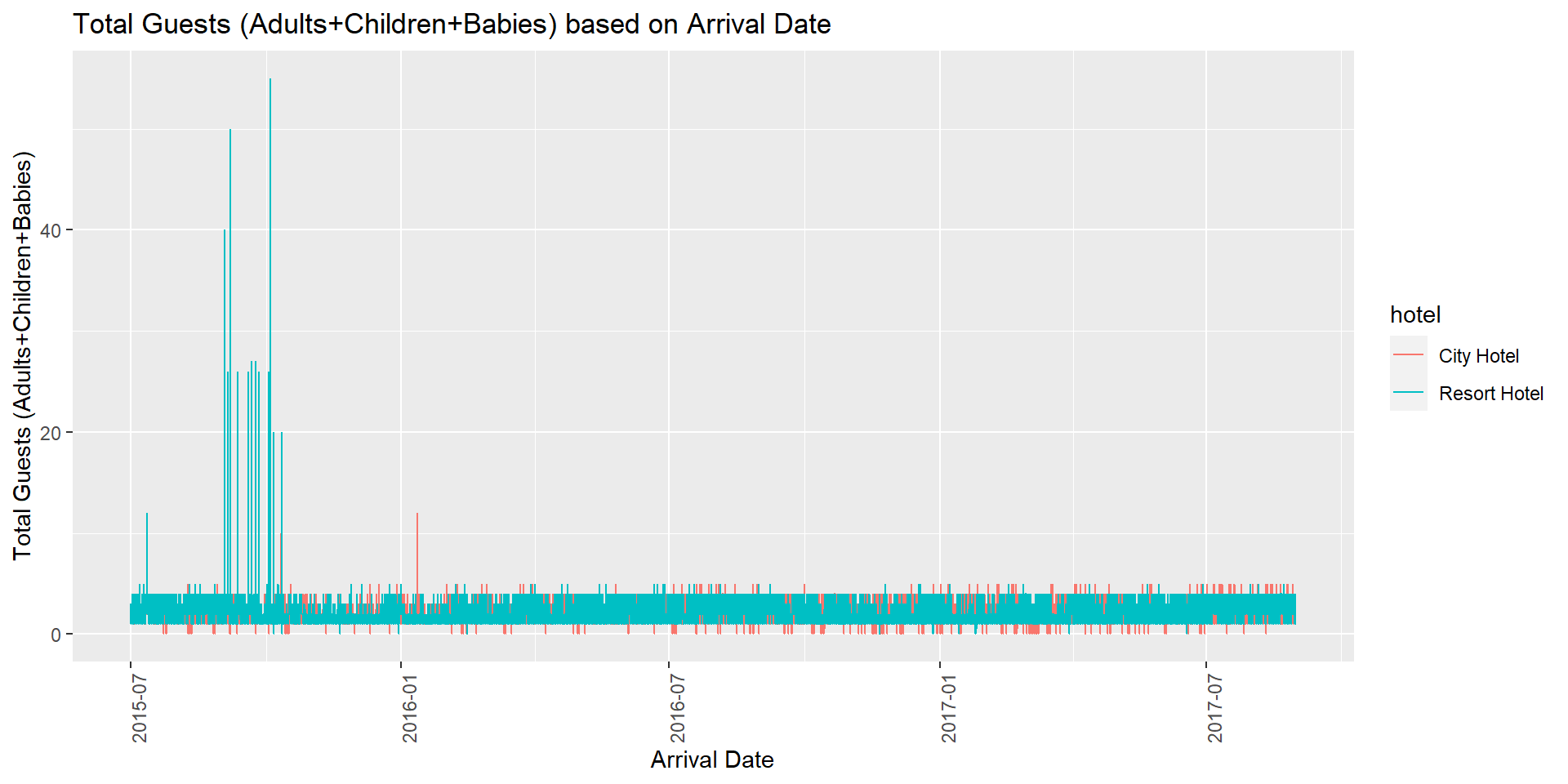
From the above visualization, we can observe that the data points are overlapping and congested as the time series is on a daily basis. This makes it difficult to arrive at any insights. In order to make the trends more clear, I decided to group by the dataset on hotel and arrival_date and summarized the sum of demand and adr.
grouped_hotel_data <- hotel_data%>%
  select(hotel, demand, arrival_date, adr)%>%
  group_by(hotel, arrival_date)%>%
  summarise(guest_total = sum(demand, na.rm=TRUE), adr_total = sum(adr, na.rm = TRUE))
grouped_hotel_data
# A tibble: 1,586 × 4
# Groups: hotel [2]
hotel arrival_date guest_total adr_total
<chr> <date> <dbl> <dbl>
1 City Hotel 2015-07-01 143 7442.
2 City Hotel 2015-07-02 96 3158.
3 City Hotel 2015-07-03 28 1184.
4 City Hotel 2015-07-04 72 2442
5 City Hotel 2015-07-05 15 532.
6 City Hotel 2015-07-06 59 1995.
7 City Hotel 2015-07-07 35 1254.
8 City Hotel 2015-07-08 79 2490.
9 City Hotel 2015-07-09 92 2952.
10 City Hotel 2015-07-10 19 647.
# … with 1,576 more rowsNext, I plotted a line plot using the grouped_hotel_data to represent the Total Guests count based on Arrival Date grouped by hotel.
# Line plot representing the Total Guests count based on Arrival Date .
ggplot(grouped_hotel_data, aes(y=guest_total, x = arrival_date, group = hotel, color = hotel)) +
  geom_line() +
  labs(title = "Total Guests (Adults+Children+Babies) based on Arrival Date",
       y = "Total Guests (Adults+Children+Babies)", x = "Arrival Date") +
  theme(axis.text.x=element_text(angle=90, hjust=1))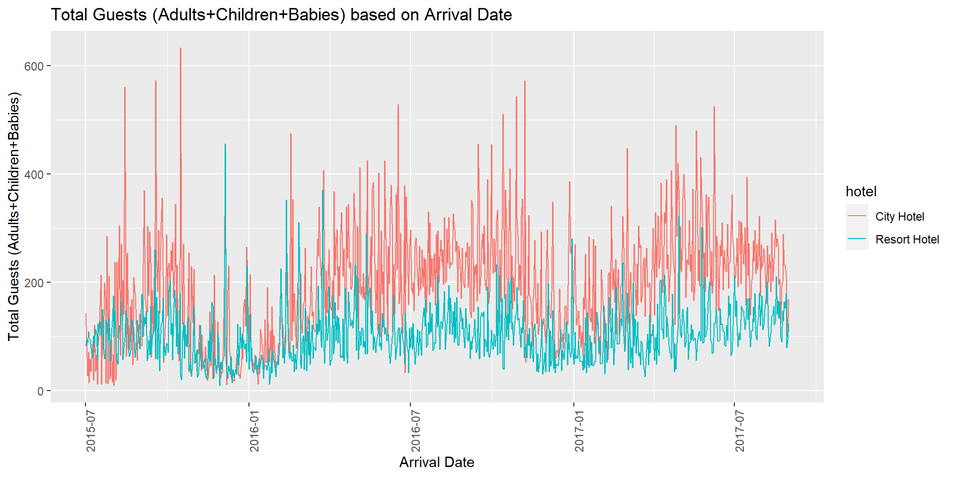
From the above visualization, we can observe that for the City Hotel, the months September and October had the highest number of guests as this is the best time to visit Portugal during Fall when the weather is warm and the crowd is relatively less compared to Summer. In general, for both the hotels, May and June had high demand (children and babies in particular) as this is the best time to stay in resort during Summer and enjoy outdoor activities with family. Hence, hotel management can price the rooms accordingly during peak season and off-season. For most of the months, City Hotel has more total guests than Resort Hotel.
Then, I plotted a line plot using the grouped_hotel_data to represent the Total ADR based on Arrival Date grouped by hotel.
# Line plot representing the Total ADR based on Arrival Date .
ggplot(grouped_hotel_data, aes(y=adr_total, x = arrival_date, group = hotel, color = hotel)) +
  geom_line() +
  labs(title = "Total ADR based on Arrival Date",
       y = "Total ADR", x = "Arrival Date") +
  theme(axis.text.x=element_text(angle=90, hjust=1))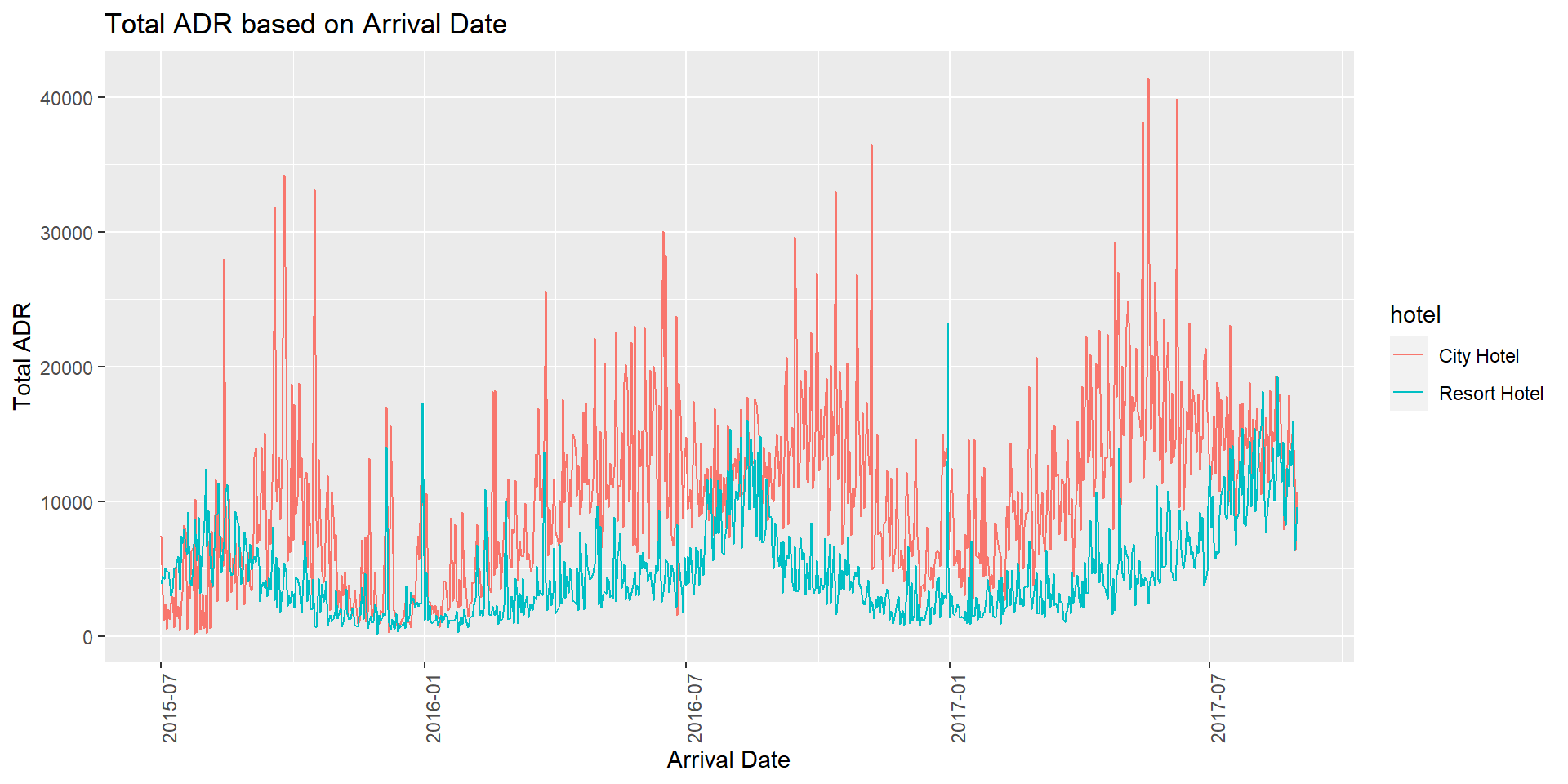
From the above visualization, we can observe that for all 3 years, the Resort Hotel has similar ADR as the City Hotel during August month. This may be because August is the best time to stay in resort during Summer and enjoy outdoor activities. Families tend to visit the Resort Hotel more during summer break with their kids and children. For most months of the year, City Hotel has more total ADR than Resort Hotel.
Visualizing Part-Whole Relationships
For visualizing Part-Whole Relationships, I plotted Grouped Bar graph and Stacked Bar graph.
# Grouped Bar graph representing the distribution of meal for hotels.

ggplot(hotel_data, aes(x = meal, fill = hotel)) +
  geom_bar(position="dodge") +
  labs(title = "Distribution of Meal preference for Hotels",
       y = "Count", x = "Meal")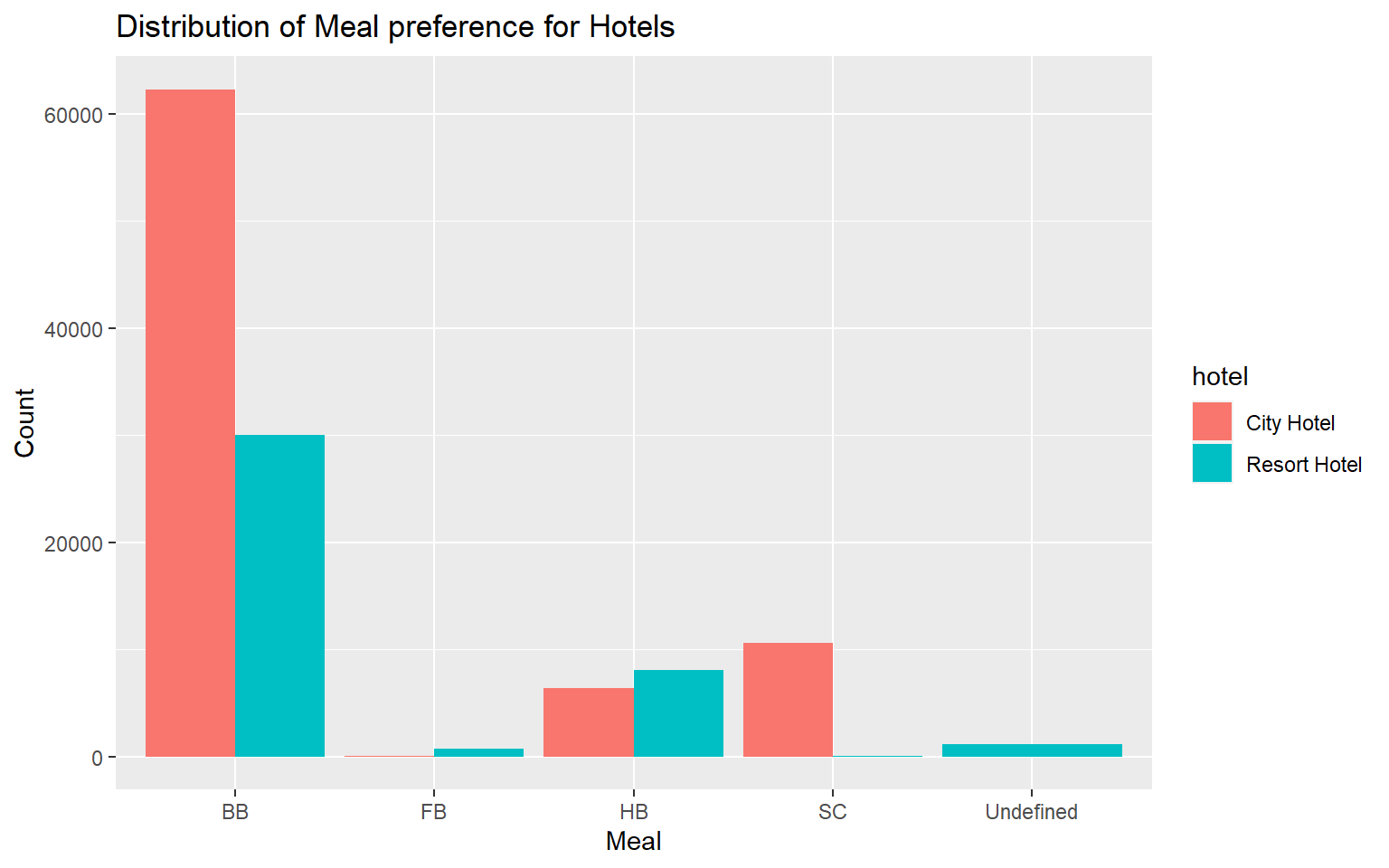
The above visualization depicts the distribution of meal preference of the guests grouped by hotel. I chose a grouped bar graph as it allows us to compare the preference of different meal types by the guests. The grouped bar graph shows how the hotel variable changes within each meal type. The taller a bar is, the larger the count of meal type. Grouped bar graph also allows us to compare both the hotels side by side. From the above visualization, we can say that BB (Bed & Breakfast) meal type is preferred by most guests in both the hotels. We can do further analysis on the data to understand why BB is the most preferred meal type. One reason may be that families with kids and children prefer BB as it is less trouble. The order of preferred meal type for City Hotel is BB, SC, HB and FB.
# Stacked Bar graph representing the distribution of Deposit Type for hotels.

ggplot(hotel_data, aes(x = deposit_type, fill = hotel)) +
  geom_bar() +
  labs(title = "Distribution of Deposit Type for Hotels",
       y = "Count", x = "Deposit Type")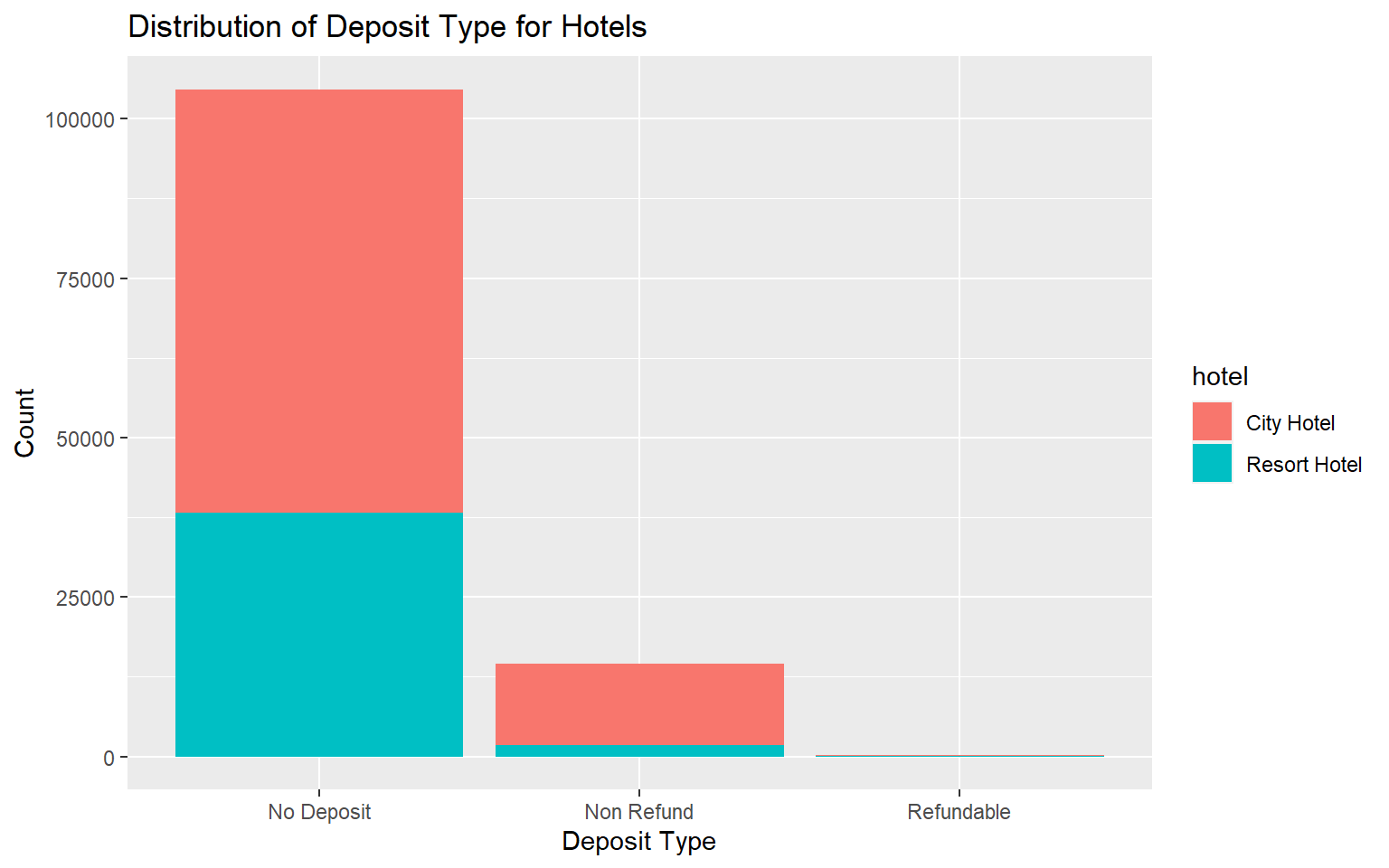
The above visualization depicts the distribution of deposit type grouped by hotel. I chose a stacked bar graph as it allows us to compare the percentage of each data point to the overall value. The taller a bar is, the larger the count of deposit type. The stacked bar graph above shows the different deposit types and the proportion of hotel for each deposit type. From the above visualization, we can say that both the hotels have “No Deposit” deposit type for most of the bookings made. City hotel does not have any bookings with “Refundable” deposit type. City Hotel has more “No Deposit” and “Non Refund” deposit type than Resort Hotel. This makes sense as we have more hotel booking observations for City Hotel compared to Resort Hotel.