library(tidyverse)
library(lubridate)
library(ggplot2)

knitr::opts_chunk$set(echo = TRUE, warning=FALSE, message=FALSE)
Challenge 7 Solutions
challenge_7
hotel_bookings
Visualizing Multiple Dimensions
Challenge Overview
Working with the Hotel data set as I had previously tidied it.
Read in data
# Reading in data
h_book <- read_csv("_data/hotel_bookings.csv", show_col_types = FALSE)
h_book
# A tibble: 119,390 × 32
hotel is_ca…¹ lead_…² arriv…³ arriv…⁴ arriv…⁵ arriv…⁶ stays…⁷ stays…⁸ adults
<chr> <dbl> <dbl> <dbl> <chr> <dbl> <dbl> <dbl> <dbl> <dbl>
1 Resor… 0 342 2015 July 27 1 0 0 2
2 Resor… 0 737 2015 July 27 1 0 0 2
3 Resor… 0 7 2015 July 27 1 0 1 1
4 Resor… 0 13 2015 July 27 1 0 1 1
5 Resor… 0 14 2015 July 27 1 0 2 2
6 Resor… 0 14 2015 July 27 1 0 2 2
7 Resor… 0 0 2015 July 27 1 0 2 2
8 Resor… 0 9 2015 July 27 1 0 2 2
9 Resor… 1 85 2015 July 27 1 0 3 2
10 Resor… 1 75 2015 July 27 1 0 3 2
# … with 119,380 more rows, 22 more variables: children <dbl>, babies <dbl>,
# meal <chr>, country <chr>, market_segment <chr>,
# distribution_channel <chr>, is_repeated_guest <dbl>,
# previous_cancellations <dbl>, previous_bookings_not_canceled <dbl>,
# reserved_room_type <chr>, assigned_room_type <chr>, booking_changes <dbl>,
# deposit_type <chr>, agent <chr>, company <chr>, days_in_waiting_list <dbl>,
# customer_type <chr>, adr <dbl>, required_car_parking_spaces <dbl>, …Briefly describe the data
The following dataset has 119390 observations and 32 different fields. This is basically the data from two hotels - City Hotel & Resort Hotel. Each entry corresponds to a booking made by a customer. There are various information that are recorded with each booking. It includes the arrival date, number of days of stay, meal, type of room reserved, customer type, reservation status, number of adult/children and many more. The data consists of entries from countries all over the world.
Tidy Data (as needed)
In country, there are entries called NULL, which can be removed as it may not be useful for the analysis.
# in country we can see that there is a field call NULL that can be removed
table(h_book$country)
  ABW   AGO   AIA   ALB   AND   ARE   ARG   ARM   ASM   ATA   ATF   AUS   AUT
    2   362     1    12     7    51   214     8     1     2     1   426  1263
  AZE   BDI   BEL   BEN   BFA   BGD   BGR   BHR   BHS   BIH   BLR   BOL   BRA
   17     1  2342     3     1    12    75     5     1    13    26    10  2224
  BRB   BWA   CAF   CHE   CHL   CHN   CIV   CMR    CN   COL   COM   CPV   CRI
    4     1     5  1730    65   999     6    10  1279    71     2    24    19
  CUB   CYM   CYP   CZE   DEU   DJI   DMA   DNK   DOM   DZA   ECU   EGY   ESP
    8     1    51   171  7287     1     1   435    14   103    27    32  8568
  EST   ETH   FIN   FJI   FRA   FRO   GAB   GBR   GEO   GGY   GHA   GIB   GLP
   83     3   447     1 10415     5     4 12129    22     3     4    18     2
  GNB   GRC   GTM   GUY   HKG   HND   HRV   HUN   IDN   IMN   IND   IRL   IRN
    9   128     4     1    29     1   100   230    35     2   152  3375    83
  IRQ   ISL   ISR   ITA   JAM   JEY   JOR   JPN   KAZ   KEN   KHM   KIR   KNA
   14    57   669  3766     6     8    21   197    19     6     2     1     2
  KOR   KWT   LAO   LBN   LBY   LCA   LIE   LKA   LTU   LUX   LVA   MAC   MAR
  133    16     2    31     8     1     3     7    81   287    55    16   259
  MCO   MDG   MDV   MEX   MKD   MLI   MLT   MMR   MNE   MOZ   MRT   MUS   MWI
    4     1    12    85    10     1    18     1     5    67     1     7     2
  MYS   MYT   NAM   NCL   NGA   NIC   NLD   NOR   NPL  NULL   NZL   OMN   PAK
   28     2     1     1    34     1  2104   607     1   488    74    18    14
  PAN   PER   PHL   PLW   POL   PRI   PRT   PRY   PYF   QAT   ROU   RUS   RWA
    9    29    40     1   919    12 48590     4     1    15   500   632     2
  SAU   SDN   SEN   SGP   SLE   SLV   SMR   SRB   STP   SUR   SVK   SVN   SWE
   48     1    11    39     1     2     1   101     2     5    65    57  1024
  SYC   SYR   TGO   THA   TJK   TMP   TUN   TUR   TWN   TZA   UGA   UKR   UMI
    2     3     2    59     9     3    39   248    51     5     2    68     1
  URY   USA   UZB   VEN   VGB   VNM   ZAF   ZMB   ZWE
   32  2097     4    26     1     8    80     2     4
h_book <- h_book %>%
filter(!(country == "NULL"))Two fields, Agents and Company have numerical values in them, but have the datatype marked as character. These NULL entries can be changed to NA and the datatype can be changed to numeric. Also, the arrival date in year, month and date can be combined into a single field called as arrival date.
# combining the arrival date into a single field
# to find the total number of guests in the hotel - add adults, children and babies

h_book_mut <- h_book %>%
  mutate(arrival_date = str_c(arrival_date_day_of_month,
                              arrival_date_month,
                              arrival_date_year, sep="/"),
         arrival_date = dmy(arrival_date),
         total_guests = adults + children + babies) %>%
  select(-c(arrival_date_day_of_month,arrival_date_year))

h_book_mut
# A tibble: 118,902 × 32
hotel is_ca…¹ lead_…² arriv…³ arriv…⁴ stays…⁵ stays…⁶ adults child…⁷ babies
<chr> <dbl> <dbl> <chr> <dbl> <dbl> <dbl> <dbl> <dbl> <dbl>
1 Resort… 0 342 July 27 0 0 2 0 0
2 Resort… 0 737 July 27 0 0 2 0 0
3 Resort… 0 7 July 27 0 1 1 0 0
4 Resort… 0 13 July 27 0 1 1 0 0
5 Resort… 0 14 July 27 0 2 2 0 0
6 Resort… 0 14 July 27 0 2 2 0 0
7 Resort… 0 0 July 27 0 2 2 0 0
8 Resort… 0 9 July 27 0 2 2 0 0
9 Resort… 1 85 July 27 0 3 2 0 0
10 Resort… 1 75 July 27 0 3 2 0 0
# … with 118,892 more rows, 22 more variables: meal <chr>, country <chr>,
# market_segment <chr>, distribution_channel <chr>, is_repeated_guest <dbl>,
# previous_cancellations <dbl>, previous_bookings_not_canceled <dbl>,
# reserved_room_type <chr>, assigned_room_type <chr>, booking_changes <dbl>,
# deposit_type <chr>, agent <chr>, company <chr>, days_in_waiting_list <dbl>,
# customer_type <chr>, adr <dbl>, required_car_parking_spaces <dbl>,
# total_of_special_requests <dbl>, reservation_status <chr>, …# mutating the datatype of the agent and company field from char to numeric
h_book_mut <- h_book_mut %>%
mutate(across(c(agent, company),~ replace(.,str_detect(., "NULL"), NA))) %>% mutate_at(vars(agent, company),as.numeric)
is.numeric(h_book_mut$agent)[1] TRUEis.numeric(h_book_mut$company)[1] TRUEVisualization with Multiple Dimensions
I had previously used only one two dimensions to visualize this dataset. I can add an additional dimension of the category of hotel to see the guest count arrival rate between “City Hotel” and “Resort Hotel”.
Firstly, I want to see how many guests are arriving over a period of time on a daily basis for each hotel separately.
plot1_data <- h_book_mut %>% select(hotel, total_guests, arrival_date) %>%
  group_by(hotel, arrival_date) %>%
  summarise(net_guests = sum(total_guests, na.rm=TRUE))

plot1_data
# A tibble: 1,586 × 3
# Groups: hotel [2]
hotel arrival_date net_guests
<chr> <date> <dbl>
1 City Hotel 2015-07-01 143
2 City Hotel 2015-07-02 96
3 City Hotel 2015-07-03 28
4 City Hotel 2015-07-04 72
5 City Hotel 2015-07-05 15
6 City Hotel 2015-07-06 59
7 City Hotel 2015-07-07 35
8 City Hotel 2015-07-08 79
9 City Hotel 2015-07-09 92
10 City Hotel 2015-07-10 19
# … with 1,576 more rows# finding the date ranges of the arrival date of this data
summary(plot1_data$arrival_date) Min. 1st Qu. Median Mean 3rd Qu. Max.
"2015-07-01" "2016-01-15" "2016-07-31" "2016-07-31" "2017-02-14" "2017-08-31" p <- ggplot(plot1_data, aes(x=arrival_date, y=net_guests, color = hotel)) + ggtitle("Guest Count Vs. Arrival Date Trend: Jul 2015 - Jun 2016") +
geom_line() +
labs(y="Net Guests", x ="Date", color="Hotel") + theme(axis.text.x=element_text(angle=60, hjust=1)) +
scale_x_date(date_labels = "%Y %b %d", date_minor_breaks = "1 month", limit=c(as.Date("2015-07-01"),as.Date("2016-07-01")))
p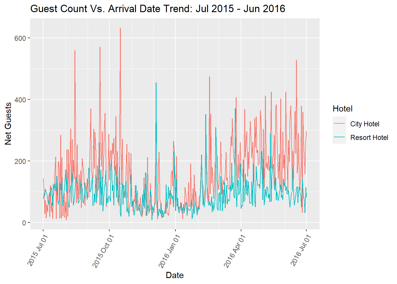
From the above plot, we can see a general trend that the number of incoming guests for the Resort Hotel are lower than that of the City Hotel. But during the first and last week of December and February, we can see that the number of incoming guests for Resort Hotel does peak higher than the City Hotel. This case can also be seen during the last week of March. These periods usually correspond to the Holiday period, where in this can be one indicator that people, prefer the Resort Hotel to the City Hotel.
Next we can try to find out during which months the total number of guests peak between the two hotels.
plot2_data <- h_book_mut %>% select(hotel, arrival_date_month, total_guests) %>%
  group_by(hotel, arrival_date_month) %>%
  summarise(net_guests = sum(total_guests, na.rm=TRUE))

plot2_data <- plot2_data %>% mutate(month = case_when(
  arrival_date_month == "January" ~ 1,
  arrival_date_month == "February" ~ 2,
  arrival_date_month == "March" ~ 3,
  arrival_date_month == "April" ~ 4,
  arrival_date_month == "May" ~ 5,
  arrival_date_month == "June" ~ 6,
  arrival_date_month == "July" ~ 7,
  arrival_date_month == "August" ~ 8,
  arrival_date_month == "September" ~ 9,
  arrival_date_month == "October" ~ 10,
  arrival_date_month == "November" ~ 11,
  arrival_date_month == "December" ~ 12,
  TRUE ~ NA_real_
)) %>% arrange(month)

plot2_data$month <-as.character(plot2_data$month)

plot2_data
# A tibble: 24 × 4
# Groups: hotel [2]
hotel arrival_date_month net_guests month
<chr> <chr> <dbl> <chr>
1 City Hotel January 6721 1
2 Resort Hotel January 3733 1
3 City Hotel February 9376 2
4 Resort Hotel February 5848 2
5 City Hotel March 12333 3
6 Resort Hotel March 6031 3
7 City Hotel April 15101 4
8 Resort Hotel April 6847 4
9 City Hotel May 15464 5
10 Resort Hotel May 6978 5
# … with 14 more rowsp <- ggplot(plot2_data, aes(fill=hotel,x=reorder(month, sort(as.numeric(month))), y=net_guests)) +
geom_bar(position="dodge", stat="identity") + labs(y="Number of Guests", x="Months", title="Monthly Trend of Number of Guests") + scale_fill_discrete(name = "Hotel")
p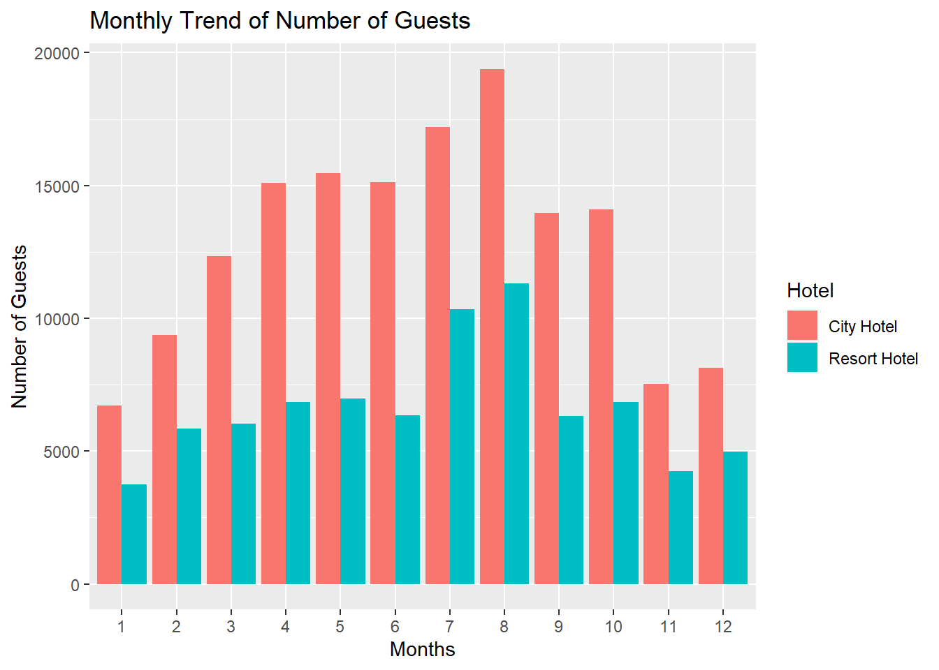
From the above visualization we can see that for City Hotel, the distribution is fairly normal. However for the Resort Hotel, the distribution is somewhat uniform through all the months, with smaller peaks during the months of July and August.
Next, I want to find the average price per night for different rooms in both the hotels and also look at how the prices vary on a monthly basis. There are 9 room types (from A-L). First I group by room type and find the mean adr and then I group by the hotels.
plot3_data <- h_book_mut %>% select(hotel, arrival_date_month, assigned_room_type, adr) %>%
  group_by(hotel, arrival_date_month, assigned_room_type) %>%
  summarise(net_adr = mean(adr, na.rm=TRUE)) %>% mutate(month = case_when(
  arrival_date_month == "January" ~ 1,
  arrival_date_month == "February" ~ 2,
  arrival_date_month == "March" ~ 3,
  arrival_date_month == "April" ~ 4,
  arrival_date_month == "May" ~ 5,
  arrival_date_month == "June" ~ 6,
  arrival_date_month == "July" ~ 7,
  arrival_date_month == "August" ~ 8,
  arrival_date_month == "September" ~ 9,
  arrival_date_month == "October" ~ 10,
  arrival_date_month == "November" ~ 11,
  arrival_date_month == "December" ~ 12,
  TRUE ~ NA_real_
)) %>% arrange(month)

plot3_data
# A tibble: 205 × 5
# Groups: hotel, arrival_date_month [24]
hotel arrival_date_month assigned_room_type net_adr month
<chr> <chr> <chr> <dbl> <dbl>
1 City Hotel January A 78.5 1
2 City Hotel January B 77.3 1
3 City Hotel January D 92.8 1
4 City Hotel January E 109. 1
5 City Hotel January F 137. 1
6 City Hotel January G 144. 1
7 City Hotel January K 44.2 1
8 Resort Hotel January A 44.8 1
9 Resort Hotel January B 34.9 1
10 Resort Hotel January C 50.1 1
# … with 195 more rowsp <- ggplot(plot3_data, aes(fill=assigned_room_type,x=reorder(month, sort(as.numeric(month))), y=net_adr)) +
geom_bar(position="dodge", stat="identity") + labs(y="Mean ADR", x="Months", title="ADR by Room Type and Hotel through the Months") + scale_fill_discrete(name = "Room Type") + facet_wrap( ~ hotel)
p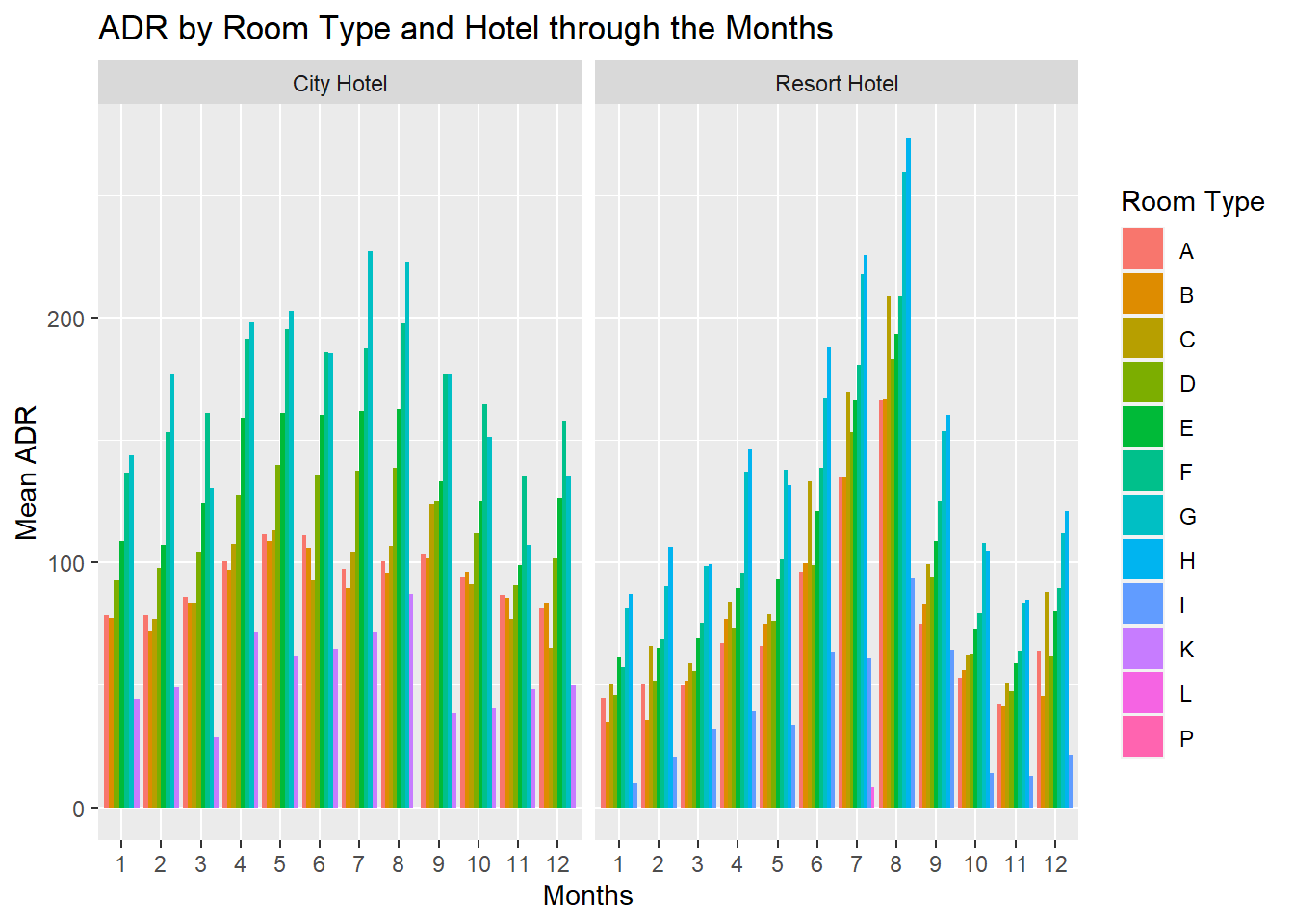
The above plot is to compare the prices of different rooms between the two hotels across various months. Generally we can see that the prices of the rooms tend to peak in the month of July and August for both the hotels. From the previous plot, it was seen that the number of guests are also high during this time. This could be probably be one of the reasons why the prices shoot up during those months. While the prices for the different rooms are fairly the same throughout the different months for City Hotel. Whereas for Resort Hotel, the prices for the different rooms follow a normal distribution.