Challenge 2

challenge_2

emma_narkewicz

birds

fao stat

In this challenge I completed data wrangling on the Birds FAO data set using group() and summarise() and summary statistic functions.

Author

Emma Narkewicz

Published

September 26, 2022

Code

library(tidyverse)

knitr::opts_chunk$set(echo = TRUE, warning=FALSE, message=FALSE)

Challenge Overview

Today’s challenge is to

read in a data set, and describe the data using both words and any supporting information (e.g., tables, etc)
provide summary statistics for different interesting groups within the data, and interpret those statistics

Read in the Data

I selected thebirds.csv for this Challenge set to push myself.

Code

#Making sure I have the right library open
library(tidyverse)
#Reading in my selected data set and remove codes, element, and domain columns
Birds <- read_csv("_data/birds.csv") %>%
  select(-c(contains("Code"), Element, Domain, Flag))

Birds

# A tibble: 30,977 × 6
   Area        Item      Year Unit      Value `Flag Description`
   <chr>       <chr>    <dbl> <chr>     <dbl> <chr>             
 1 Afghanistan Chickens  1961 1000 Head  4700 FAO estimate      
 2 Afghanistan Chickens  1962 1000 Head  4900 FAO estimate      
 3 Afghanistan Chickens  1963 1000 Head  5000 FAO estimate      
 4 Afghanistan Chickens  1964 1000 Head  5300 FAO estimate      
 5 Afghanistan Chickens  1965 1000 Head  5500 FAO estimate      
 6 Afghanistan Chickens  1966 1000 Head  5800 FAO estimate      
 7 Afghanistan Chickens  1967 1000 Head  6600 FAO estimate      
 8 Afghanistan Chickens  1968 1000 Head  6290 Official data     
 9 Afghanistan Chickens  1969 1000 Head  6300 FAO estimate      
10 Afghanistan Chickens  1970 1000 Head  6000 FAO estimate      
# … with 30,967 more rows

Code

#Replace value and unit columns with Number_of_Birds columns, creating Birds_Clean data set
Birds_Clean = transmute(Birds,
  Area = Area,
  Item = Item,
  Year = Year,
  Number_of_Birds = Value*1000,
  `Flag Description` = `Flag Description`
)  


Birds_Clean

# A tibble: 30,977 × 5
   Area        Item      Year Number_of_Birds `Flag Description`
   <chr>       <chr>    <dbl>           <dbl> <chr>             
 1 Afghanistan Chickens  1961         4700000 FAO estimate      
 2 Afghanistan Chickens  1962         4900000 FAO estimate      
 3 Afghanistan Chickens  1963         5000000 FAO estimate      
 4 Afghanistan Chickens  1964         5300000 FAO estimate      
 5 Afghanistan Chickens  1965         5500000 FAO estimate      
 6 Afghanistan Chickens  1966         5800000 FAO estimate      
 7 Afghanistan Chickens  1967         6600000 FAO estimate      
 8 Afghanistan Chickens  1968         6290000 Official data     
 9 Afghanistan Chickens  1969         6300000 FAO estimate      
10 Afghanistan Chickens  1970         6000000 FAO estimate      
# … with 30,967 more rows

The original “Birds” data frame had 30977 rows and 14 columns. A clean “Birds_Clean” data frame was created for analysis by removing the redundant or extraneous code, Element, Domain, and Flag columns. Additionally, the Unit and Value columns were replaced with the Number_of_Birds column , created by converting values in units of 1000 Head to the total number of birds in the easy to work with units of birds.

Describe the data

Code

#calculating min, median, mean, and max Number_of_Birds column, removing na from dataset
summarise(Birds_Clean, min_birds = min(Number_of_Birds, na.rm = TRUE), median_birds = median(Number_of_Birds, na.rm = TRUE), mean_birds = mean(Number_of_Birds, na.rm = TRUE), max_birds = max(Number_of_Birds, na.rm = TRUE))

# A tibble: 1 × 4
  min_birds median_birds mean_birds   max_birds
      <dbl>        <dbl>      <dbl>       <dbl>
1         0      1800000  99410630. 23707134000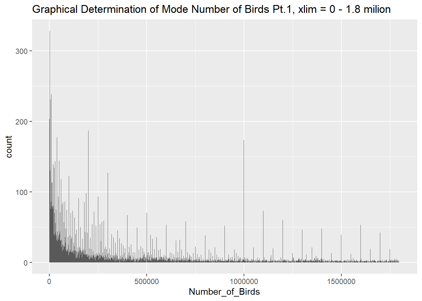

Code

#Creating a bar chart of Values to identify the mode, using the xlim() function to graph from min-max of data
ggplot(Birds_Clean, aes(Number_of_Birds)) + geom_bar() + xlim(0, 1800000) + labs(title = "Graphical Determination of Mode Number of Birds Pt.1, xlim = 0 - 1.8 milion" )

Code

#narrowing in to identify mode
ggplot(Birds_Clean, aes(Number_of_Birds))+ geom_bar() + xlim(0,8000) + labs(title = "Graphical Determination of Mode Number of Birds Pt.2, xlim = 0 - 8,000" )

Code

#Highest number of birds
Birds_Clean%>%
  arrange(desc(Number_of_Birds)) %>%
  select(Area, Item, Number_of_Birds, Year, `Flag Description`) %>%
  slice(1:100)

# A tibble: 100 × 5
   Area  Item     Number_of_Birds  Year `Flag Description`                      
   <chr> <chr>              <dbl> <dbl> <chr>                                   
 1 World Chickens     23707134000  2018 Aggregate, may include official, semi-o…
 2 World Chickens     23212565000  2017 Aggregate, may include official, semi-o…
 3 World Chickens     22826754000  2016 Aggregate, may include official, semi-o…
 4 World Chickens     21678753000  2015 Aggregate, may include official, semi-o…
 5 World Chickens     21118803000  2014 Aggregate, may include official, semi-o…
 6 World Chickens     20953583000  2013 Aggregate, may include official, semi-o…
 7 World Chickens     20489756000  2012 Aggregate, may include official, semi-o…
 8 World Chickens     20244638000  2010 Aggregate, may include official, semi-o…
 9 World Chickens     19950281000  2011 Aggregate, may include official, semi-o…
10 World Chickens     19720796000  2009 Aggregate, may include official, semi-o…
# … with 90 more rows

Code

#Fewest number of birds
Birds_Clean %>%
  arrange(Number_of_Birds)%>%
  select(Area, Item, Number_of_Birds, Year, `Flag Description`) %>%
  slice(1:100)

# A tibble: 100 × 5
   Area                 Item                   Number_of_Birds  Year Flag Desc…¹
   <chr>                <chr>                            <dbl> <dbl> <chr>      
 1 Aruba                Chickens                             0  1991 Official d…
 2 Aruba                Chickens                             0  1992 Official d…
 3 Bermuda              Ducks                                0  1976 Official d…
 4 Bermuda              Ducks                                0  1977 FAO estima…
 5 Bermuda              Ducks                                0  1978 FAO estima…
 6 Bermuda              Ducks                                0  1979 FAO estima…
 7 Bermuda              Ducks                                0  1980 Official d…
 8 Bermuda              Ducks                                0  1981 FAO estima…
 9 Bermuda              Ducks                                0  1982 FAO estima…
10 China, Hong Kong SAR Geese and guinea fowls               0  1993 Official d…
# … with 90 more rows, and abbreviated variable name ¹`Flag Description`

The bird data set was put together by the [United Nation’s Food and Agricultural Organization] (https://www.fao.org/about/en) as part of their larger statistical data base created for the purposes of tracking and defeating hunger internationally. The clean “Birds_Clean” data frame has 5 columns: Area, Item, Year, Number_of_Birds, and Flag Description.

The Area column contains the location of the bird-stock, ranging from estimates of the total bird-stock world-wide, for entire continents, or for individual countries. There are 248 unique areas in the data frame. By using the arrange(), select(), and slice() functions it was determined that the with “World” having the most number of birds of any area followed by Asia, while the areas with the fewest total number of birds tended to be islands.

The Item column refers to which of the 5 types of bird-stocks is being measured in each row: chickens, ducks, geese or fowl, pigeons/other birds, or turkeys. Chickens were the most common item type (42.7% of all items) and pigeons, other birds was the least common item type (3.8% of all items).

The Year column is self explanatory and spans 58 years ranging from 1961 through 2018. Year seemed to contribute to the size of number of birds, with the top 10 most number of birds all occurring between the 10 year of 2009 through 2018. This suggests the size of bird stocks is likely increasing over time.

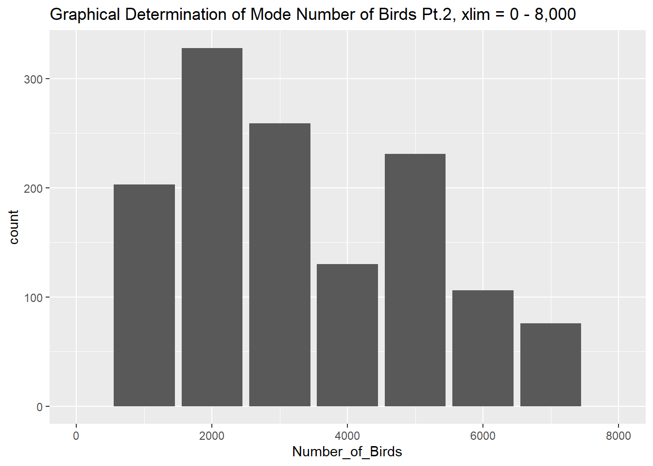
The “Number_of_Birds” column describes the number of birds for each item type in the specified location and year. The minimum number of birds was 0, the median number of birds was 1.8 million, the mean number of birds was 99.4 million, and the maximum number of birds is 23.7 billion. The mode number of birds was 2,000, which was determined graphically. 1036 rows had N/A for Number_of_Birds meaning that value was missing from the data set.

Lastly, the Flag Description column refers to the origin of each data and can be used to gauge the data_quality with 6 different flag descriptions: Aggregate data, Data not available, FAO data based on imputation, FAO estimate, Official data, and Unofficial data. Using the FAO flag descriptions from the table of top 50 number of birds, the data for largest total number of birds were determined using aggregate data.

Provide Grouped Summary Statistics, Explain, & Interpret

Conduct some exploratory data analysis, using dplyr commands such as group_by(), select(), filter(), and summarise(). Find the central tendency (mean, median, mode) and dispersion (standard deviation, mix/max/quantile) for different subgroups within the data set.

Area and Total Number of Birds

After reading in, previewing, and describing the Birds_Clean data set, I decided it would be interesting to look at the relationship between Area and Number of Birds. When looking at tables of the largest and smallest bird-stocks, area seemed to significantly factor into size of bird stocks, so decided to look more closely at this.

Code

#Using group_by(), select(), summarize(), and arrange() to generate a table of Area of mean and median total number of birds descending by the median value
Birds_Clean %>%
  group_by(Area)%>%
  select(Area, Number_of_Birds) %>%
  summarise( mean_birds= mean(Number_of_Birds, na.rm=TRUE), median_birds = median(Number_of_Birds, na.rm = TRUE)) %>%
  arrange(desc(median_birds))

# A tibble: 248 × 3
   Area                      mean_birds median_birds
   <chr>                          <dbl>        <dbl>
 1 World                    2565908193.    328049000
 2 China, mainland           981424759.    320500000
 3 USSR                      413426790.    247250000
 4 United States of America  536970356.    240219000
 5 Nigeria                   104694569.    116370000
 6 Asia                     1246442041.    103030000
 7 Eastern Asia              679408245.     96090000
 8 India                     177719707.     68307500
 9 Americas                  856355944.     66923500
10 Indonesia                 368163560.     60005500
# … with 238 more rows

Using the piping, group_by(), select(),summarize(), and arrange() functions, I created a table of the mean and median values per area, descending by median. I arranged the data-set by median as it is less likely to be skewed by outliers than the mean. The mean number of birds for the Area of the world was 2.57 billion, which is almost 8 times larger than the median number of birds for the world, which was 328 million. The areas with highest median total number of birds, starting with the highest are: World, “China, mainland, USSR, United States of America, Nigeria, Asia, Eastern Asia, India, Americas, and Indonesia. It made sense that the World has the highest median value of all areas, but I was surprised that the China (mainland), USSR, the USA, and Nigeria all had a higher area median value than Asia, when considering that the highest 50 total number of birds were all based in the area of World or Asia. A confusing finding is that the median Value for the USA is higher than the median value for”the Americas” which the USA is a part of, so I’d be curious to know if something brought the median down for the Americas. Along those lines, it would be interesting to know what feature of Nigeria make it have a higher median number of birds than its continent of Africa.

Descending, the 10 lowest median values by area were Liechtenstein, Papua New Guinea, Saint Helena, Ascension and Tristan da Cunha, Jordan, Cayman Islands, Saint Pierre and Miquelon, Nauru, Tokelau, Falkland Islands (Malvinas), and Aruba. It follows earlier patterns observed from the lowest 50 values that islands comprised the majority of area with low values, as the climate of small islands is likely not conducive for poultry-stock. Liechtenstein and Jordan do not follow this pattern, as a small German town and a West-African country, and it would be interesting to learn why they are on this list. These ten areas with the lowest median values ranged from 0-12,000 birds which means these areas likely need to rely heavily on poultry imports or other protein sources.

Code

#Using group_by(), select(), summarize(), and arrange() to generate a table of Area of min, max, sd, IQR, and range of number of birds,  descending by range/

Birds_Clean %>%
  group_by(Area)%>%
  select(Area, Number_of_Birds)%>%
  summarise(min_birds = min(Number_of_Birds, na.rm = TRUE), max_birds = max(Number_of_Birds, na.rm =TRUE), range_birds = max_birds-min_birds, sd_birds= sd(Number_of_Birds, na.rm=TRUE), IQR_birds = IQR(Number_of_Birds, na.rm = TRUE)) %>%
   arrange(desc(range_birds))

# A tibble: 248 × 6
   Area               min_birds   max_birds range_birds    sd_birds IQR_birds
   <chr>                  <dbl>       <dbl>       <dbl>       <dbl>     <dbl>
 1 World               12068000 23707134000 23695066000 5297664399. 985833500
 2 Asia                 3408000 13630958000 13627550000 2776107770. 926803250
 3 Eastern Asia           93000  5884748000  5884655000 1372882881. 665932250
 4 Americas              553000  5796289000  5795736000 1539315549. 545152000
 5 China, mainland     15000000  5274475000  5259475000 1436610595. 599500000
 6 South-eastern Asia     42000  3862039000  3861997000  680622395. 157789500
 7 Southern Asia         350000  2786706000  2786356000  565733859. 103088000
 8 South America         199000  2611687000  2611488000  615392924. 112260000
 9 Europe               2417000  2486932000  2484515000  777666805.  97111000
10 Indonesia            5300000  2384147000  2378847000  579077970. 488042250
# … with 238 more rows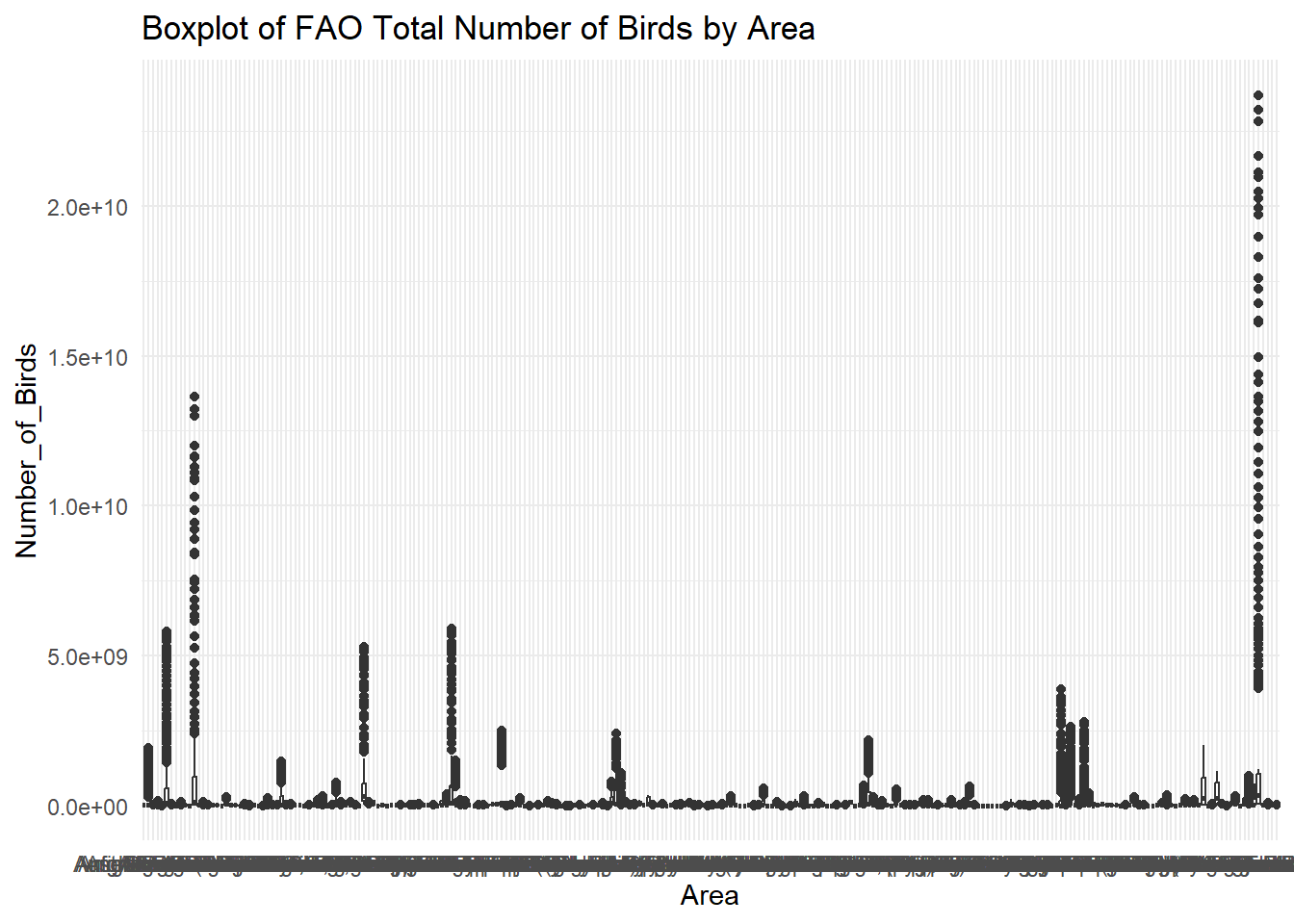

Code

#Creating a boxplot of Number of Birds by Area
ggplot(Birds_Clean, aes(Area, Number_of_Birds)) + geom_boxplot() + theme_minimal() + labs(title = "Boxplot of FAO Total Number of Birds by Area")

Once again using the piping, group_by(), select(),summarize(), and arrange(), I created a table of the minimum, maximum, range, standard deviation, IQR of number birds for each area, sorted in descending order by range, to look at the dispersion of the data. I also created a boxplot graphing the Number_of_Birds vs. Area to better visualize the data.

Looking at this table, the Americas has the 4th largest range of number of birds for all areas in the data frame, at ~5.8 billion. The USA had the 12th largest range of number birds for all areas at ~2 billion. The Americas has a minimum number of birds of 553,000, whereas the USA had a 6 times higher minimum number of birds of 3.4 million. While the Americas have a higher maximum number of birds at ~ 5.8 billion vs USA’s maximum number of birds of ~2 billion, the differences in minimum numbers of birds and range helps explains why the USA has a higher median number of birds than the USA.

Looking at the world – which had the largest range and IQR for number of birds – we can see that despite area contributing to the number of birds, there is still a large range in number of birds for each area. This means that area alone cannot explain all of the variation in number_of_birds. Therefore, I decided to look at the relationship between time (as measured by Year) and the number of birds.

Year and Total Number of Birds

Using the piping, group_by(), and summarise() functions, I created a table of the mean and median of the total number of birds grouped by year. I sorted the table descending by mean number of birds to get average data for each year.

Code

#Create table of number of birds by year

Birds_Clean %>%
  group_by(Year)%>%
  summarise(avg_birds = mean(Number_of_Birds, na.rm = TRUE), med_birds = median(Number_of_Birds, na.rm = TRUE))%>%
   arrange(desc(avg_birds))

# A tibble: 58 × 3
    Year  avg_birds med_birds
   <dbl>      <dbl>     <dbl>
 1  2018 182869178.   2830500
 2  2017 179185690.   2764000
 3  2016 176522797.   2798000
 4  2015 168025068.   2734500
 5  2014 163800537.   2687500
 6  2013 162940899.   2574000
 7  2012 159889568.   2352000
 8  2010 158516613.   2200000
 9  2011 155450242.   2367000
10  2009 154204552.   2207000
# … with 48 more rows

Looking at this table, the data follows the expected trend almost perfectly - with time the average total number of birds in a stock increases. The top 10 higher average number of birds in a stock is from the 10 most recent year 2009-2018. In fact, the top 10 average number of birds in a stock is in perfect chronological data, with the exception of more avg_birds in 2011 than 2010. It is clear from this table that over time the average number of birds increases. So while the world will have the largest bird_stock, the world in 2018 will likely have a larger bird stock than the world in 2000.

Code

#Graph of Birds by year FAO STAT data
ggplot(Birds_Clean, aes(Year, Number_of_Birds)) + geom_point() + theme_minimal() + labs(title = "Total Number of Birds by Year")

Code

#Graph of Birds by year FAO STAT data 0-1billion
ggplot(Birds_Clean, aes(Year, Number_of_Birds)) + geom_point() + theme_minimal() + ylim(0, 1000000000) + labs(title = "Total Number of Birds by Year, ylim = 0-1billion")

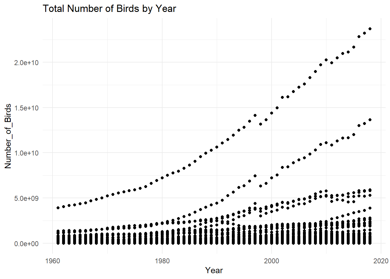
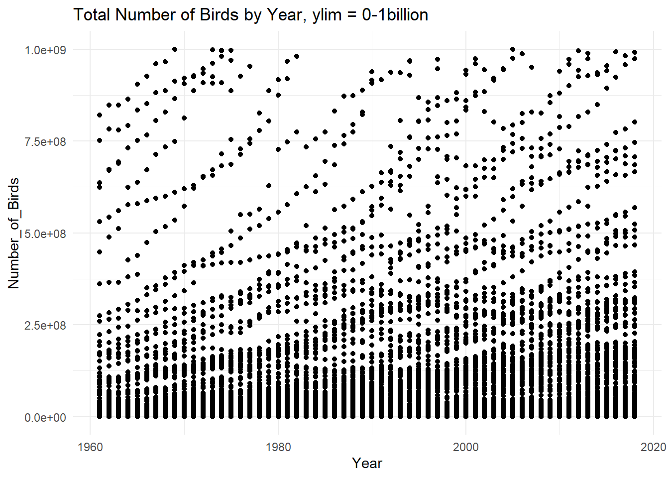
Looking at the above graph of Number_of_Birds vs. Years, it is once again clear that the number of bird stocks increase by time. With this scale appears to be 3 distinct trend-lines, with most data concentrated near the bottom of the y-axis. Viewing the second graph zoomed in on the y axis from 0-1billion using ylim(), while its its crowded at the bottom of the y-axis but at the top of the graph you can see the trend of number of birds increasing with time (Year).

Item, Year, and Number of Birds

So far, I have examined the impact of area and year on number of birds, but not examined the item. To do so I created a table using the pivot_wider() function to examine the average number of birds for each of the 5 types of Item at 2 points of time 50 years apart, 1968 and 2018. I used kable() to rename the column headings and add commas to the data in the table.

Code

#creating a table using the pivot_wider solution modeling the example pivot_wider solution we reviewed in class and using knitr::kable() to add commas and rename the column headings.
t1<-Birds_Clean %>%
  filter(Year %in% c(1968, 2018))%>%
  group_by(Year, Item)%>%
  summarise(avg_birds = mean(Number_of_Birds, na.rm=TRUE))%>%
  pivot_wider(names_from = Year, values_from = c(avg_birds))

knitr::kable(t1,
             digits=0,format.args = list(big.mark = ","),
             col.names = c("Bird Type", "Average Birds in 1968", "Average Birds in 2018"))

Bird Type	Average Birds in 1968	Average Birds in 2018
Chickens	91,003,212	396,772,130
Ducks	9,166,421	38,132,814
Geese and guinea fowls	3,245,371	19,236,000
Pigeons, other birds	2,839,529	5,484,714
Turkeys	7,959,256	17,288,444

Looking at the table, for every bird type, the average number of birds increased from 1968 to 2018. In this time span, the average number of chickens increased by 4.36 times, the average number of ducks increased by 4.16 times, the average number of geese and guinea fowls increased by 6.77 times, the average number of pigeons and other birds increased by 1.93 times, and the average number of turkeys increased by 2.17 times. The average number of chickens remains much higher than the other bird types over the 50 years, almost reaching 400 million in 2018. The average number of pigeons and other birds remains relatively low compared to the other bird types, not even reaching 5.5 million birds in 2018. Even when factoring in Item (Bird Type), the trend of total number of birds increasing over time for a bird stock remains.

Conclusion

By wrangling the FAO STAT bird data in R using dply functions I observed that larger areas generally had larger bird-stocks. Additionally, I observed that bird-stocks increased over time – even when accounting for different bird types (Item).