Challenge 2 Instructions

challenge_2

railroads

faostat

hotel_bookings

Author

Matthew Norberg

Published

September 17, 2022

Code

library(tidyverse)

knitr::opts_chunk$set(echo = TRUE, warning=FALSE, message=FALSE)

Challenge Overview

Today’s challenge is to

read in a data set, and describe the data using both words and any supporting information (e.g., tables, etc)
provide summary statistics for different interesting groups within the data, and interpret those statistics

Read in the Data

Read in one (or more) of the following data sets, available in the posts/_data folder, using the correct R package and command.

railroad*.csv or StateCounty2012.xls ⭐
FAOstat*.csv or birds.csv ⭐⭐⭐
hotel_bookings.csv ⭐⭐⭐⭐

Code

# Read in the hotel bookings data set
df <- read_csv('./_data/hotel_bookings.csv')

Add any comments or documentation as needed. More challenging data may require additional code chunks and documentation.

Describe the data

Using a combination of words and results of R commands, can you provide a high level description of the data? Describe as efficiently as possible where/how the data was (likely) gathered, indicate the cases and variables (both the interpretation and any details you deem useful to the reader to fully understand your chosen data).

First, let’s look at the columns in the data set and the first few entries to get an idea of what each instance of the data is describing.

Code

spec(df)

cols(
  hotel = col_character(),
  is_canceled = col_double(),
  lead_time = col_double(),
  arrival_date_year = col_double(),
  arrival_date_month = col_character(),
  arrival_date_week_number = col_double(),
  arrival_date_day_of_month = col_double(),
  stays_in_weekend_nights = col_double(),
  stays_in_week_nights = col_double(),
  adults = col_double(),
  children = col_double(),
  babies = col_double(),
  meal = col_character(),
  country = col_character(),
  market_segment = col_character(),
  distribution_channel = col_character(),
  is_repeated_guest = col_double(),
  previous_cancellations = col_double(),
  previous_bookings_not_canceled = col_double(),
  reserved_room_type = col_character(),
  assigned_room_type = col_character(),
  booking_changes = col_double(),
  deposit_type = col_character(),
  agent = col_character(),
  company = col_character(),
  days_in_waiting_list = col_double(),
  customer_type = col_character(),
  adr = col_double(),
  required_car_parking_spaces = col_double(),
  total_of_special_requests = col_double(),
  reservation_status = col_character(),
  reservation_status_date = col_date(format = "")
)

Code

head(df)

# A tibble: 6 × 32
  hotel   is_ca…¹ lead_…² arriv…³ arriv…⁴ arriv…⁵ arriv…⁶ stays…⁷ stays…⁸ adults
  <chr>     <dbl>   <dbl>   <dbl> <chr>     <dbl>   <dbl>   <dbl>   <dbl>  <dbl>
1 Resort…       0     342    2015 July         27       1       0       0      2
2 Resort…       0     737    2015 July         27       1       0       0      2
3 Resort…       0       7    2015 July         27       1       0       1      1
4 Resort…       0      13    2015 July         27       1       0       1      1
5 Resort…       0      14    2015 July         27       1       0       2      2
6 Resort…       0      14    2015 July         27       1       0       2      2
# … with 22 more variables: children <dbl>, babies <dbl>, meal <chr>,
#   country <chr>, market_segment <chr>, distribution_channel <chr>,
#   is_repeated_guest <dbl>, previous_cancellations <dbl>,
#   previous_bookings_not_canceled <dbl>, reserved_room_type <chr>,
#   assigned_room_type <chr>, booking_changes <dbl>, deposit_type <chr>,
#   agent <chr>, company <chr>, days_in_waiting_list <dbl>,
#   customer_type <chr>, adr <dbl>, required_car_parking_spaces <dbl>, …

The output above shows that each row in the data set is describing an instance of a hotel booking. For each booking, we are recording 32 data parameters as described by the columns. Additionally, we can see that some of the entries have a value of “NULL”. For instance, the first row of the data set has an agent and company listed as “NULL”. This is probably used to describe instances in which an travel agent or travel company was not used. The following code creates a data frame containing all the rows that have a “NULL” value.

Code

NULLS <- df %>% filter_all(any_vars(. %in% c('NULL')))
head(NULLS)

# A tibble: 6 × 32
  hotel   is_ca…¹ lead_…² arriv…³ arriv…⁴ arriv…⁵ arriv…⁶ stays…⁷ stays…⁸ adults
  <chr>     <dbl>   <dbl>   <dbl> <chr>     <dbl>   <dbl>   <dbl>   <dbl>  <dbl>
1 Resort…       0     342    2015 July         27       1       0       0      2
2 Resort…       0     737    2015 July         27       1       0       0      2
3 Resort…       0       7    2015 July         27       1       0       1      1
4 Resort…       0      13    2015 July         27       1       0       1      1
5 Resort…       0      14    2015 July         27       1       0       2      2
6 Resort…       0      14    2015 July         27       1       0       2      2
# … with 22 more variables: children <dbl>, babies <dbl>, meal <chr>,
#   country <chr>, market_segment <chr>, distribution_channel <chr>,
#   is_repeated_guest <dbl>, previous_cancellations <dbl>,
#   previous_bookings_not_canceled <dbl>, reserved_room_type <chr>,
#   assigned_room_type <chr>, booking_changes <dbl>, deposit_type <chr>,
#   agent <chr>, company <chr>, days_in_waiting_list <dbl>,
#   customer_type <chr>, adr <dbl>, required_car_parking_spaces <dbl>, …

The original dataframe had 119,390 rows while the new dataframe called ‘NULLS’ created above has 119,173 rows. This shows that the vast majority of the rows in the dataset have at least one “NULL” value (99.8%).

Let’s find out if there are any missing values in the data set. The code chunk below finds the columns that contain NA.

Code

# Identify columns containing NA
colnames(df)[apply(df, 2, anyNA)]

[1] "children"

The ‘children’ column of the data set contains values that are not available. We can use the filter function to identify the rows of the data set that contain NA.

Code

# Find the rows in the data set containing NA
filter(df, is.na(children))

# A tibble: 4 × 32
  hotel   is_ca…¹ lead_…² arriv…³ arriv…⁴ arriv…⁵ arriv…⁶ stays…⁷ stays…⁸ adults
  <chr>     <dbl>   <dbl>   <dbl> <chr>     <dbl>   <dbl>   <dbl>   <dbl>  <dbl>
1 City H…       1       2    2015 August       32       3       1       0      2
2 City H…       1       1    2015 August       32       5       0       2      2
3 City H…       1       1    2015 August       32       5       0       2      3
4 City H…       1       8    2015 August       33      13       2       5      2
# … with 22 more variables: children <dbl>, babies <dbl>, meal <chr>,
#   country <chr>, market_segment <chr>, distribution_channel <chr>,
#   is_repeated_guest <dbl>, previous_cancellations <dbl>,
#   previous_bookings_not_canceled <dbl>, reserved_room_type <chr>,
#   assigned_room_type <chr>, booking_changes <dbl>, deposit_type <chr>,
#   agent <chr>, company <chr>, days_in_waiting_list <dbl>,
#   customer_type <chr>, adr <dbl>, required_car_parking_spaces <dbl>, …

The data set has 119,390 rows. The code above shows that 4 of those rows contain entries that are not available. Since only a small proportion of rows contain entries that are not available, it is likely safe to remove them. Running the code cell below will remove the rows listed above and generate a clean data set.

Code

df <- na.omit(df)

An analysis of the ‘arrival_data_year’ column reveals that the data was collected over the course of three years from 2015 to 2017. This can be shown with the following R command: summary(df$arrival_date_year). Additionally, we can see that the tibble contains information about hotel bookings from all over the world, as evident by the ‘country’ column. The code chunk below reveals that there are 167 unique countries in the data set. Note that although the tibble generated below has 168 rows, one of those rows is for those data entries whose country is not known. In these cases, the country is listed as “NULL”.

Code

countries <- select(df, country) %>%
  group_by(country) %>%
  summarise(TotalBookings = n()) %>%
  arrange(desc(TotalBookings))

countries

# A tibble: 178 × 2
   country TotalBookings
   <chr>           <int>
 1 PRT             48586
 2 GBR             12129
 3 FRA             10415
 4 ESP              8568
 5 DEU              7287
 6 ITA              3766
 7 IRL              3375
 8 BEL              2342
 9 BRA              2224
10 NLD              2104
# … with 168 more rows

Code

summary(countries$TotalBookings)

    Min.  1st Qu.   Median     Mean  3rd Qu.     Max. 
    1.00     2.00    12.50   670.71    74.75 48586.00

Code

countryHist <- ggplot(countries, aes(x=TotalBookings)) + geom_histogram(colour = "black", fill = "white", bins = 40)
print(countryHist + ggtitle("Hotel Booking Frequency per Country vs Number of Countries") + 
        labs(x = "Number of hotel bookings", y = "Number of countries"))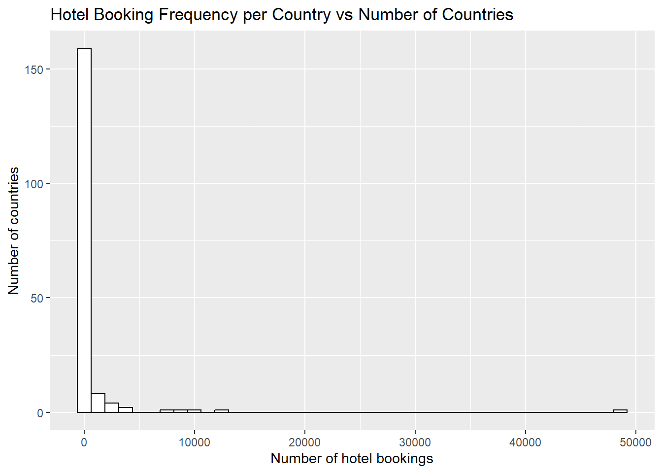

An analysis on the tibble shows that Portugal has the most hotel bookings in the data set. Additionally, the summary command below reveals that the average number of bookings is 670.71 and the median number of bookings is 12.5. The histogram derived from the count of each country further reveals that the number of bookings per country is skewed.

The categorical nature of the ‘hotel’, ‘meal’, ‘reserved_room_type’, and ‘customer_type’ columns of the data set lead me to believe that the data was collected by a singular Hotel Company that has locations all over the world. They have categorized their hotels as being in one of two possible categories, “Resort Hotel” and “City Hotel”. It seems unlikely that multiple hotel companies would use the same categorization. Additionally, this particular hotel company has a set of meal categories, room type categories, and customer categories. I would argue that these categorization are not a standard that is being used by multiple hotels which furthers my theory that this data was collected by a singular hotel company. The code chunk below lists the possible categories for each of the aforementioned columns.

Code

unique(df$hotel)

[1] "Resort Hotel" "City Hotel"

Code

unique(df$reserved_room_type)

 [1] "C" "A" "D" "E" "G" "F" "H" "L" "P" "B"

Code

unique(df$is_repeated_guest)

[1] 0 1

Provide Grouped Summary Statistics

Conduct some exploratory data analysis, using dplyr commands such as group_by(), select(), filter(), and summarise(). Find the central tendency (mean, median, mode) and dispersion (standard deviation, mix/max/quantile) for different subgroups within the data set.

Let’s look at the set of hotel bookings that took place in the United States. I was interested in determining how many bookings were made in which the customer got the type of room that they requested. The code chunk below answers this question.

Code

# Get the rows that contain hotel booking information in the United States
us <- filter(df, country == "USA")

# Find the proportion of bookings where the customer got the correct room type
correctType <- us %>%
  filter(reserved_room_type == assigned_room_type) %>%
  summarise(Count = n()) / dim(us)[1]

# Display the answer
cat("The proportion of bookings where the customer got the correct room type in the United States:", correctType[[1]])

The proportion of bookings where the customer got the correct room type in the United States: 0.8874583

The data shows that most people were able to get the room type that they requested in the United States. However, I was in interested in figuring out how the United States compares to other countries in terms of accuracy of hotel bookings. The following code chunk computes the booking accuracy of all countries listed in the table and sorts them based on accuracy.

Code

# Compute the booking accuracy of each country
r <- df %>%
  group_by(country) %>%
  filter(reserved_room_type == assigned_room_type) %>%
  summarise(CorrectRoom = n()) %>%
  left_join(countries, by = "country") %>%
  mutate(PercentCorrect = CorrectRoom / TotalBookings) %>%
  arrange(desc(PercentCorrect))

# Display the results
head(r)

# A tibble: 6 × 4
  country CorrectRoom TotalBookings PercentCorrect
  <chr>         <int>         <int>          <dbl>
1 AIA               1             1              1
2 ALB              12            12              1
3 AND               7             7              1
4 ARM               8             8              1
5 ASM               1             1              1
6 ATA               2             2              1

Code

summary(r)

   country           CorrectRoom      TotalBookings     PercentCorrect  
 Length:173         Min.   :    1.0   Min.   :    1.0   Min.   :0.3333  
 Class :character   1st Qu.:    2.0   1st Qu.:    3.0   1st Qu.:0.8765  
 Mode  :character   Median :   14.0   Median :   14.0   Median :0.9231  
                    Mean   :  603.9   Mean   :  690.1   Mean   :0.9107  
                    3rd Qu.:   67.0   3rd Qu.:   80.0   3rd Qu.:1.0000  
                    Max.   :42477.0   Max.   :48586.0   Max.   :1.0000

The results from the code chunk above show that there are many countries with perfect booking accuracy. Furthermore, the average accuracy was 91%. Therefore, the United States is below average in terms of hotel booking accuracy.

In addition to hotel booking accuracy, I was also interested in the total number of nights stayed that each booking incurred in the United States. The data set has two columns for the number of nights stayed: ‘stays_in_weekend_nights’ and ‘stays_in_week_nights’. Here, I am defining the total number of nights to be the sum of those two children. Specifically, I wanted to know if the total number of nights stayed in the hotel is influenced by whether or not the booking included children and babies. The code chunk below computes the average number of nights and the median number of nights for each (children, babies) pairing in the data set for hotel bookings in the US.

Code

# Compute central tendency and dispersion for total number of nights in the united states grouped by children and babies
# Total number of nights = weekend nights + week nights
temp <- us %>%
  mutate(total_nights = stays_in_weekend_nights + stays_in_week_nights) %>%
  group_by(children, babies) %>%
  summarise(AverageNights = mean(total_nights), NumOccurences = n(), MedianNights = median(total_nights))

# Display the information
temp

# A tibble: 5 × 5
# Groups:   children [4]
  children babies AverageNights NumOccurences MedianNights
     <dbl>  <dbl>         <dbl>         <int>        <dbl>
1        0      0          2.76          1871          2  
2        0      1          3.17             6          3.5
3        1      0          2.51            83          2  
4        2      0          3.16           132          3  
5        3      0          1.6              5          1

The results in the table above show that offspring status of a hotel booking does not seem to have an impact on the average number of nights stayed in the hotel.

Lastly, I was interested in the lead time attribute for bookings in the United States. I wanted to determine if some months are more popular than others and therefore have a larger lead time. The following code chunk computes averaged lead time grouped by ‘arrival_date_month’ to determine which months are the most popular.

Code

# Lets look at lead time statistics grouped by month to see if some months are more popular
leadTime <- us %>%
  group_by(arrival_date_month) %>%
  summarise(AverageLeadTime = mean(lead_time), 
            sdLeadTime = sd(lead_time), 
            maxLeadTime = max(lead_time), 
            minLeadTime = min(lead_time))

leadTime

# A tibble: 12 × 5
   arrival_date_month AverageLeadTime sdLeadTime maxLeadTime minLeadTime
   <chr>                        <dbl>      <dbl>       <dbl>       <dbl>
 1 April                         76.5       74.2         317           0
 2 August                       101.       104.          504           0
 3 December                      58.7       63.3         237           0
 4 February                      24.9       35.8         240           0
 5 January                       35.3       47.3         343           0
 6 July                         104.        96.4         476           0
 7 June                          89.0       77.0         423           0
 8 March                         54.3       56.6         286           0
 9 May                           85.2       80.8         340           0
10 November                      48.4       51.4         260           0
11 October                       67.4       78.6         241           0
12 September                     56.6       73.5         542           0

The results above show that the summer months seem to have the highest average lead time while some of the winter months have the fewest lead times. This may indicate that the summer months are the most popular times to go on vacation.

Explain and Interpret

Be sure to explain why you choose a specific group. Comment on the interpretation of any interesting differences between groups that you uncover. This section can be integrated with the exploratory data analysis, just be sure it is included.

I choose to look at hotel bookings in the United States to do my analysis. The first portion of my analysis looked at hotel booking accuracy in the United States versus the other countries in the data set. I was surprised that the United States is below the average accuracy in the data set.

I also looked at the total number of nights for each booking the United States. I wanted to know if having children or babies included in the hotel booking impacted how long people stay. The idea was interesting, but the results indicated that having children and babies included in the booking did not seem to impact total stay.

Lastly, I looked at the amount of lead time in hotel bookings for the United States in order to see which months were the most popular. Unsurprisingly, the summer months were among the most popular and the least popular were winter months.