Challenge 2 Kristin Abijaoude

Code

library(tidyverse)
library(dplyr)

knitr::opts_chunk$set(echo = TRUE, warning=FALSE, message=FALSE)

Code

railroads <- read_csv("_data/railroad_2012_clean_county.csv")
railroads

# A tibble: 2,930 × 3
   state county               total_employees
   <chr> <chr>                          <dbl>
 1 AE    APO                                2
 2 AK    ANCHORAGE                          7
 3 AK    FAIRBANKS NORTH STAR               2
 4 AK    JUNEAU                             3
 5 AK    MATANUSKA-SUSITNA                  2
 6 AK    SITKA                              1
 7 AK    SKAGWAY MUNICIPALITY              88
 8 AL    AUTAUGA                          102
 9 AL    BALDWIN                          143
10 AL    BARBOUR                            1
# … with 2,920 more rows

This dataset is county-level data from censuses across 2930 counties with at least one railroad employee. Each row has information about the county name, the state that the county is in, and the total number of railroad employees in said county. The information is likely collected from the 2012 US Census.

Code

summary(railroads)

    state              county          total_employees  
 Length:2930        Length:2930        Min.   :   1.00  
 Class :character   Class :character   1st Qu.:   7.00  
 Mode  :character   Mode  :character   Median :  21.00  
                                       Mean   :  87.18  
                                       3rd Qu.:  65.00  
                                       Max.   :8207.00  

Code

## Selecting county and total employees
select(railroads, `county`, `total_employees`)

# A tibble: 2,930 × 2
   county               total_employees
   <chr>                          <dbl>
 1 APO                                2
 2 ANCHORAGE                          7
 3 FAIRBANKS NORTH STAR               2
 4 JUNEAU                             3
 5 MATANUSKA-SUSITNA                  2
 6 SITKA                              1
 7 SKAGWAY MUNICIPALITY              88
 8 AUTAUGA                          102
 9 BALDWIN                          143
10 BARBOUR                            1
# … with 2,920 more rows

Code

## Average # of employees in each state
railroads %>%
  group_by(state) %>%
  summarise(mean.employees = mean(total_employees, na.rm = TRUE))

# A tibble: 53 × 2
   state mean.employees
   <chr>          <dbl>
 1 AE               2  
 2 AK              17.2
 3 AL              63.5
 4 AP               1  
 5 AR              53.8
 6 AZ             210. 
 7 CA             239. 
 8 CO              64.0
 9 CT             324  
10 DC             279  
# … with 43 more rows

Code

## filtering counties with up to 100 railroad employees
filter(railroads,`total_employees` <= 100)

# A tibble: 2,400 × 3
   state county               total_employees
   <chr> <chr>                          <dbl>
 1 AE    APO                                2
 2 AK    ANCHORAGE                          7
 3 AK    FAIRBANKS NORTH STAR               2
 4 AK    JUNEAU                             3
 5 AK    MATANUSKA-SUSITNA                  2
 6 AK    SITKA                              1
 7 AK    SKAGWAY MUNICIPALITY              88
 8 AL    BARBOUR                            1
 9 AL    BIBB                              25
10 AL    BULLOCK                           13
# … with 2,390 more rows

Code

summarize(railroads, mean.total_employees = mean(`total_employees`, na.rm = TRUE), median.total_employees = median(`total_employees`, na.rm = TRUE), min.total_employees = min(`total_employees`, na.rm = TRUE), max.total_employees = max(`total_employees`, na.rm = TRUE), sd.total_employees = sd(`total_employees`, na.rm = TRUE), var.total_employees = var(`total_employees`, na.rm = TRUE), IQR.total_employees = IQR(`total_employees`, na.rm = TRUE))

# A tibble: 1 × 7
  mean.total_employees median.total_em…¹ min.t…² max.t…³ sd.to…⁴ var.t…⁵ IQR.t…⁶
                 <dbl>             <dbl>   <dbl>   <dbl>   <dbl>   <dbl>   <dbl>
1                 87.2                21       1    8207    284.  80449.      58
# … with abbreviated variable names ¹​median.total_employees,
#   ²​min.total_employees, ³​max.total_employees, ⁴​sd.total_employees,
#   ⁵​var.total_employees, ⁶​IQR.total_employees

There are many more counties with a lower number of total railroad employees than those with a higher number of them, which partially explains the low numbers for median and mean, and why the mean is greater than the median. The standard deviation is very high which shows there were outliers with large values, such as Cook County, IL with 8207 railroad employees.

Code

library(ggplot2)
ggplot(railroads, aes(x=state, y=total_employees)) + 
    geom_point()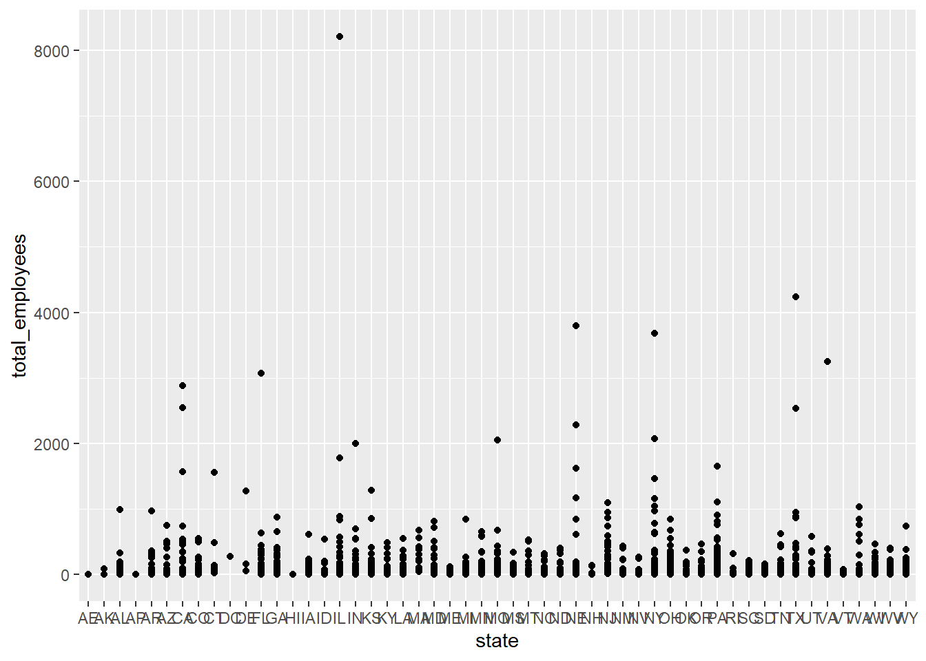

I attempted to create a scatterplot graph to display the amount of railroad employees by state, with each dot representing county. Plenty of states have counties that are more clustered, while some states have one or outlier counties, such as Illinois and New York. When you look into population density of the those states, you can see that the majority of the population lives in a particular area, while the rest of the state is relatively sparse.