Code
library(tidyverse)

knitr::opts_chunk$set(echo = TRUE, warning=FALSE, message=FALSE)library(tidyverse)
knitr::opts_chunk$set(echo = TRUE, warning=FALSE, message=FALSE)Today’s challenge is to:
pivot_longerI chose to read in the Australian Marriage Survey Data. The original data set was in an excel format with 4 sheets: Contents, Table 1, Table 2, & Explanatory Notes. I read in specifically the Table 2 sheet of Federal Election Divisions, as it includes information from the State & Territory data in Table 1.
For each federal election district, there is data for each eligible participant if there was:
A clear response, unclear response, of no response
If a response was clear, was it yes or no.
In this read in step I skipped the first 7 rows which included titles and blank row not necessary to the analysis. I assigned column names using col_names() to be able to easily identify and delete certain columns using select. I removed the blank column H, the total, and percentage columns, and response clear column. The total & percentages can be re-constructed from the other columns, and clear responses numbers are redundant to the yes and no columns (clear responses = no + yes). The original sheet had 16 columns and 191 rows. At this step in the read in, there are now 5 columns and 184 rows.
#Read In Data Pt1
library(readxl)
Aus_Marriage_Data <-read_excel("_data/australian_marriage_law_postal_survey_2017_-_response_final.xls",
        sheet = 3,
        skip = 7,
        col_names = c("District", "Yes", "Percent", "No", "Percent", "Total", "Total_Percent", "Blank", "Response_Clear", "Response_Clear_Percent", "Unclear_Response", "Unclear_Response_Percent","Non_Response", "Non_Response_Percent", "Total", "Total_Percent")) %>%
        select(!contains("Percent")) %>%
        select(!contains("Total")) %>%
        select(!contains("Blank")) %>%
        select(!contains("Response_Clear"))

Aus_Marriage_Data
# A tibble: 184 × 5
District Yes No Unclear_Response Non_Response
<chr> <dbl> <dbl> <dbl> <dbl>
1 New South Wales Divisions NA NA NA NA
2 Banks 37736 46343 247 20928
3 Barton 37153 47984 226 24008
4 Bennelong 42943 43215 244 19973
5 Berowra 48471 40369 212 16038
6 Blaxland 20406 57926 220 25883
7 Bradfield 53681 34927 202 17261
8 Calare 54091 35779 285 25342
9 Chifley 32871 46702 263 28180
10 Cook 47505 38804 229 18713
# … with 174 more rowsAt this point I have removed redundant and blanks columns and the first 7 rows, but there are still additional rows that need to be dealt with.There are 1) Total rows for divisions 2) Blank rows between divisions, 3) The bottom rows of the sheet, that contain notes, and Australia wide data.
To begin, I used the head function to remove the bottom 10 rows of the table, which contain notes and Australian based data. This left me with the total and blank rows to get rid of. I knew to use filter() function to select row but I was at a loss for how to specify which rows I wanted without the contains() starts_with() and ends_with() functions I have learned to love working with select(). After finding nothing in the R For Data Science textbook, I turned to Professor Rolfe’s Challenge 3 solutions.
The drop_na(), str_detect(), and str_starts() function were used in the Challenge 3 Solution, so I embarked on a quest to understand why these functions were applicable here.
drop_na() drop rows containing missing values.
str_detect and str_starts( ) are functions within the stringr package. str_detect() identifies the presence of pattern match in a a string and str_starts() identifies the presence of a pattern match in the beginning of a string
#Remove Notes & Australia Wide data
Aus_Marriage_Data <- head(Aus_Marriage_Data, -10) %>%
#Remove blank rows between Divisions using drop)na
   drop_na("District") %>%
#Remove total rows using function
  filter(!str_detect(District,"(Total)"))

Aus_Marriage_Data
# A tibble: 158 × 5
District Yes No Unclear_Response Non_Response
<chr> <dbl> <dbl> <dbl> <dbl>
1 New South Wales Divisions NA NA NA NA
2 Banks 37736 46343 247 20928
3 Barton 37153 47984 226 24008
4 Bennelong 42943 43215 244 19973
5 Berowra 48471 40369 212 16038
6 Blaxland 20406 57926 220 25883
7 Bradfield 53681 34927 202 17261
8 Calare 54091 35779 285 25342
9 Chifley 32871 46702 263 28180
10 Cook 47505 38804 229 18713
# … with 148 more rowsAfter removing redundant rows and columns, I now have a data set with the dimensions of 144 x 5. The 5 columns are: District_, Yes, No, Unclear_Response, and Non_Response. The district division column contains mostly districts, with the division at the top of every list of districts. Before pivoting the data, I need to separate out district and division.
This transformation was advanced for me, and required once again referencing Professor Rolfe’s Challenge 3 Solutions to accomplish it. I know how to fill missing data and how to separate a column when 2 pieces of data are in one row, but this case is neither of those. There are are no rows with missing data to fill and Division are written in a separate row than districts, as opposed to being written District_Division.
I show this out step by step to make sure I understand why each step is necessary and can apply it moving forward to other data sets when applicable.
Based on the Challenge 3 Solution, we can overcome this using case_when to first create a new Divisions column whenever a row ends with “Divisions” (e.g., New South Wales Divisions). This works, but I don’t like that this new Division column is all the way to the right, so I use relocate() to move it before District column.
#Creating new division column
Aus_Marriage <- Aus_Marriage_Data %>%
  mutate(Division = case_when(
    str_ends(District, "Divisions") ~ District)
  )%>%
  relocate(`Division`, .before = `District`)

Aus_Marriage
# A tibble: 158 × 6
Division District Yes No Uncle…¹ Non_R…²
<chr> <chr> <dbl> <dbl> <dbl> <dbl>
1 New South Wales Divisions New South Wales Divisi… NA NA NA NA
2 <NA> Banks 37736 46343 247 20928
3 <NA> Barton 37153 47984 226 24008
4 <NA> Bennelong 42943 43215 244 19973
5 <NA> Berowra 48471 40369 212 16038
6 <NA> Blaxland 20406 57926 220 25883
7 <NA> Bradfield 53681 34927 202 17261
8 <NA> Calare 54091 35779 285 25342
9 <NA> Chifley 32871 46702 263 28180
10 <NA> Cook 47505 38804 229 18713
# … with 148 more rows, and abbreviated variable names ¹Unclear_Response,
# ²Non_ResponseNext, I use the fill() function to fill the empty Division column rows. This is possible because the Division applies to all the districts in a row up until the next division.
#Fill down the divisions
Aus_Marriage <- Aus_Marriage %>%
 fill(Division)

Aus_Marriage
# A tibble: 158 × 6
Division District Yes No Uncle…¹ Non_R…²
<chr> <chr> <dbl> <dbl> <dbl> <dbl>
1 New South Wales Divisions New South Wales Divisi… NA NA NA NA
2 New South Wales Divisions Banks 37736 46343 247 20928
3 New South Wales Divisions Barton 37153 47984 226 24008
4 New South Wales Divisions Bennelong 42943 43215 244 19973
5 New South Wales Divisions Berowra 48471 40369 212 16038
6 New South Wales Divisions Blaxland 20406 57926 220 25883
7 New South Wales Divisions Bradfield 53681 34927 202 17261
8 New South Wales Divisions Calare 54091 35779 285 25342
9 New South Wales Divisions Chifley 32871 46702 263 28180
10 New South Wales Divisions Cook 47505 38804 229 18713
# … with 148 more rows, and abbreviated variable names ¹Unclear_Response,
# ²Non_ResponseThis is nifty! I now have a column of districts, and a column of divisions, which I wanted. Looking at the tibble, I still have the pesky row where the Division is in the district column and there are no response data. To get rid of this, I can use filter() and str_detect(), specifying that I want to remove any row in which the District column contains “Divisions”.
Aus_Marriage <- filter(Aus_Marriage, !str_detect(`District`, "Divisions"))

Aus_Marriage
# A tibble: 150 × 6
Division District Yes No Unclear_Response Non_Response
<chr> <chr> <dbl> <dbl> <dbl> <dbl>
1 New South Wales Divisions Banks 37736 46343 247 20928
2 New South Wales Divisions Barton 37153 47984 226 24008
3 New South Wales Divisions Bennelong 42943 43215 244 19973
4 New South Wales Divisions Berowra 48471 40369 212 16038
5 New South Wales Divisions Blaxland 20406 57926 220 25883
6 New South Wales Divisions Bradfield 53681 34927 202 17261
7 New South Wales Divisions Calare 54091 35779 285 25342
8 New South Wales Divisions Chifley 32871 46702 263 28180
9 New South Wales Divisions Cook 47505 38804 229 18713
10 New South Wales Divisions Cowper 57493 38317 315 25197
# … with 140 more rowsWoohoo! We did it. I leaned on the Challenge 3 Solutions, but was able to think critically through why I applied each step. Now lets pivot some data!
I want to pivot the Yes, No, Unclear_Response, and Non_Response columns into “Response_Type”, and “Response_Count” columns. A case would then be a response count for a response type, in a district, in a division.
I expect my pivoted data_set to have 4 columns, Division, District, Response Type, and Response_Count.
My un-pivoted data set has 150 rows and I am pivoting 4 columns.
150 * 4[1] 600I therefor expect by pivoted data set to have dimensions of 600 rows by 4 columns.
Aus_Marriage_tidy <-pivot_longer(Aus_Marriage, col = c("Yes", "No", "Unclear_Response", "Non_Response"),
                 names_to="Response_Type",
                 values_to = "Response_Count")

Aus_Marriage_tidy
# A tibble: 600 × 4
Division District Response_Type Response_Count
<chr> <chr> <chr> <dbl>
1 New South Wales Divisions Banks Yes 37736
2 New South Wales Divisions Banks No 46343
3 New South Wales Divisions Banks Unclear_Response 247
4 New South Wales Divisions Banks Non_Response 20928
5 New South Wales Divisions Barton Yes 37153
6 New South Wales Divisions Barton No 47984
7 New South Wales Divisions Barton Unclear_Response 226
8 New South Wales Divisions Barton Non_Response 24008
9 New South Wales Divisions Bennelong Yes 42943
10 New South Wales Divisions Bennelong No 43215
# … with 590 more rowsAwesome, the dimensions of the pivoted table set are indeed 600 x 4. This data set is tidy and ready to work with to perform further statistic or graphical analysis.
I tried to create a bar chart of the Response_Count of each Response_Type per division, but that did not work. You can see in the bar chart below that each Response_Type color of the bar is equal in size, whereas looking at the data, the response counts vary a lot by Response_Type. The Unclear_Response bar segments should be much smaller than the Yes, No, and Non_Response bar segments, but they appear to be equal in size here. Reviewing the R for Data Science textbook, R auto-generates the Counts in bar charts, and it seems that whatever it is using as counts is not the Response_Counts I’m looking for.
#Attempting Bar Chart of Response Count by Division

ggplot(data = Aus_Marriage_tidy) + geom_bar(mapping = aes(x=`Division`, fill = `Response_Type`)) + labs(title="Wrong Bar Chart of Australian Marriage Survey Responses by Division")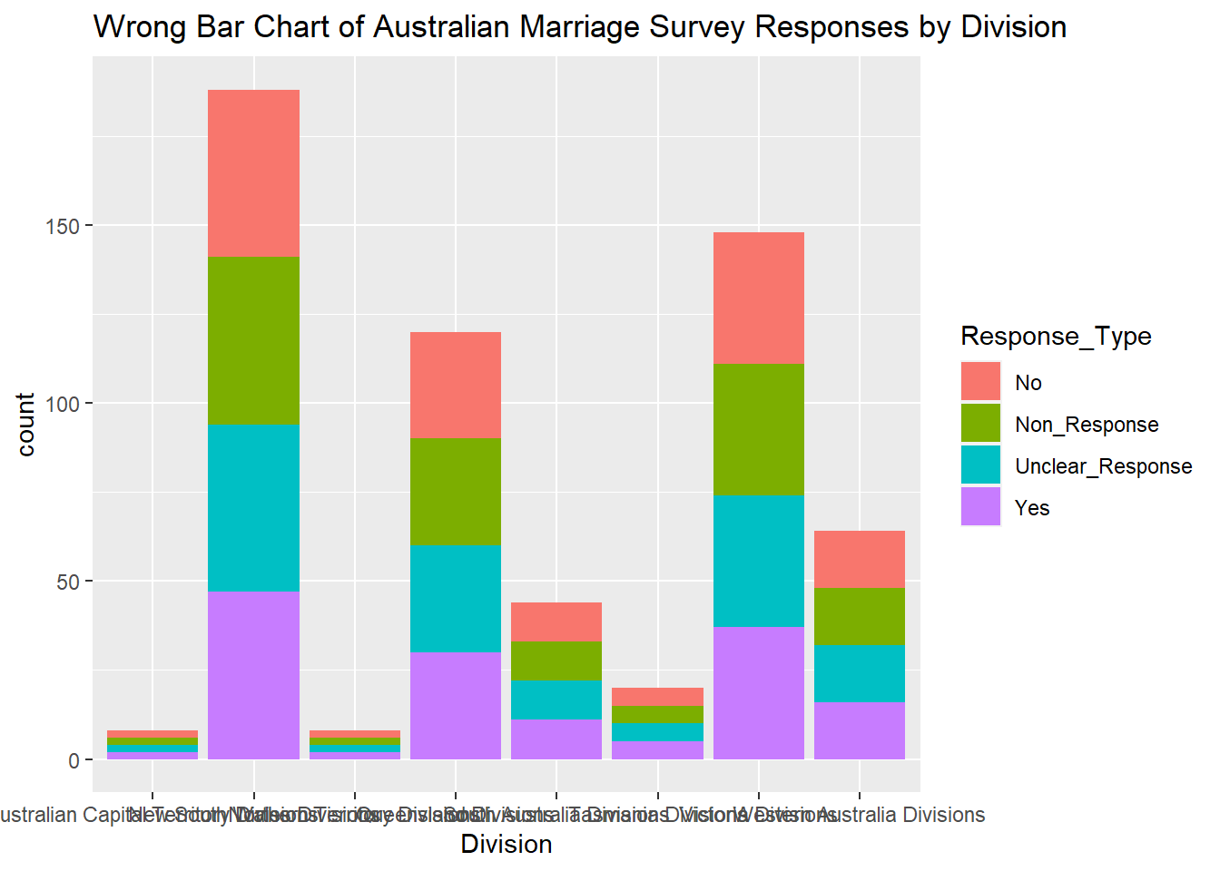
I will attempt to override the incorrect default count by setting the stat of geom_bar() from the default count to identity, allowing me to specify the y = Response_Count.
#Attempting another bar chart of Response Count by Division

ggplot(data = Aus_Marriage_tidy) + geom_bar(mapping = aes(x=`Division`, y = `Response_Count`, fill = `Response_Type`), stat = "identity") + labs(title="Correct Bar Chart of Australian Marriage Survey Responses by Division")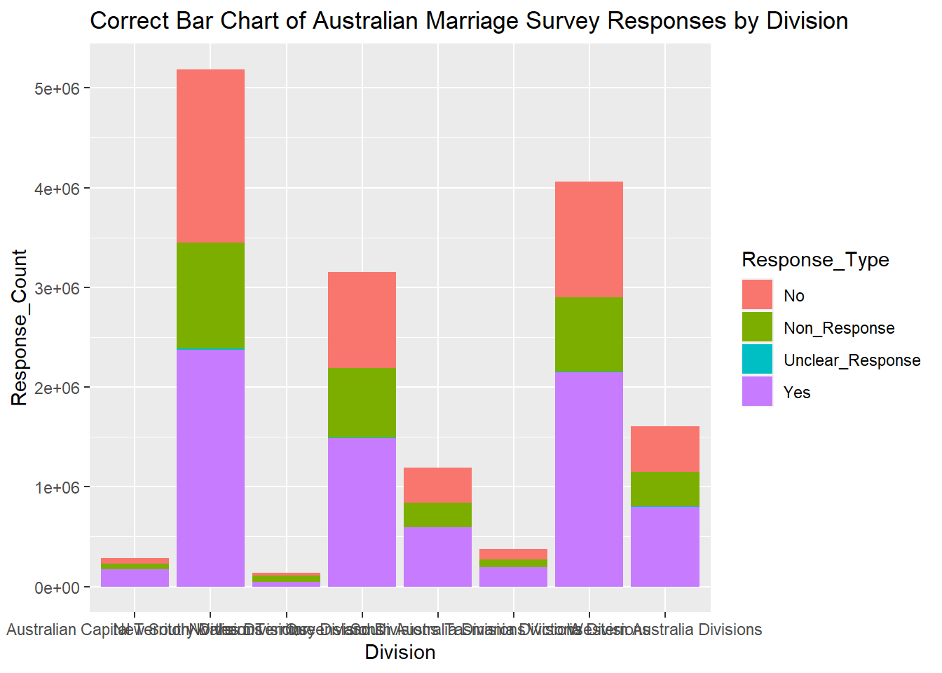
Cool, it worked! I’m glad I played around with graphing to learn I need to be wary of trusting the default bar chart stats. I can now see that in all divisions “yes” was the most popular response type, followed by no, then non_response. Unclear responses exist but make up a fraction of a percentage of all responses, and are represented as a very thin teal line on the bar chart.