Challenge 5

Introduction to Visualization

library(tidyverse)
library(ggplot2)

knitr::opts_chunk$set(echo = TRUE, warning=FALSE, message=FALSE)

Challenge Overview

Today’s challenge is to:

1. read in a data set, and describe the data set using both words and any supporting information (e.g., tables, etc)
2. tidy data (as needed, including sanity checks)
3. mutate variables as needed (including sanity checks)
4. create at least two univariate visualizations

• try to make them “publication” ready
• Explain why you choose the specific graph type

5. Create at least one bivariate visualization

• try to make them “publication” ready
• Explain why you choose the specific graph type

R Graph Gallery is a good starting point for thinking about what information is conveyed in standard graph types, and includes example R code.

(be sure to only include the category tags for the data you use!)

Read in data

• cereal.csv ⭐

cereal <- read.csv("_data/cereal.csv")
cereal<-rename(cereal, "Name" = "Cereal")

Briefly describe the data

The dataset gives information about amount of sugar and sodium in different types of cereal. We can see 20 different cereal products. The dataset contains 20 cases and 4 variables (“Cereal”, “Sodium”, “Sugar”, “Type”). There are two values for “Type”, A and C.

summary(cereal)

     Name               Sodium          Sugar           Type          
 Length:20          Min.   :  0.0   Min.   : 0.00   Length:20         
 Class :character   1st Qu.:137.5   1st Qu.: 4.00   Class :character  
 Mode  :character   Median :180.0   Median : 9.50   Mode  :character  
                    Mean   :167.0   Mean   : 8.75                     
                    3rd Qu.:202.5   3rd Qu.:12.50                     
                    Max.   :340.0   Max.   :18.00                     

Tidy Data (as needed)

I think, data is already tidy. I did not find missing data. To prepare data for visualization I am going to turn “Name” variable into factor to arrange bar chart.

cereal$Name <- as.factor(cereal$Name)
cereal <- arrange(cereal, Sugar)
library(forcats)
cereal <- cereal %>%
  mutate(Name = fct_relevel(Name, "Raisin Bran",
                            "Crackling Oat Bran",
                            "Honey Smacks",
                            "Apple Jacks",
                            "Froot Loops",
                            "Captain Crunch",
                            "Frosted Flakes",
                            "Frosted Mini Wheats",
                            "Honeycomb",
                            "Cinnamon Toast Crunch",
                            "Honey Nut Cheerios",
                            "Honey Bunches of Oats",
                            "Life",
                            "All Bran",
                            "Special K",
                            "Wheaties",
                            "Rice Krispies",
                            "Corn Flakes",
                             "Cheerios",
                            "Fiber One"))

Univariate Visualizations

1. First, I chose bar chart to visualize difference in the amount of sugar in cereals. Chart shows name of the product and amount of sugar. I think it is easy to understand information quickly from the graph.
2. As a second univariate visualization I chose histogram for values of sugar variable. Even though the number of cases is small I decided to look at distribution of values. It will help to understand if there is some tendency in amount of sugar in cereals.

ggplot(cereal, aes(x=Name, y=Sugar)) + geom_bar (stat = "identity", fill="pink", width=0.7) + coord_flip() + theme_light() + xlab("Product name") + ylab("Amount of sugar") + ggtitle("Amount of sugar in cereals")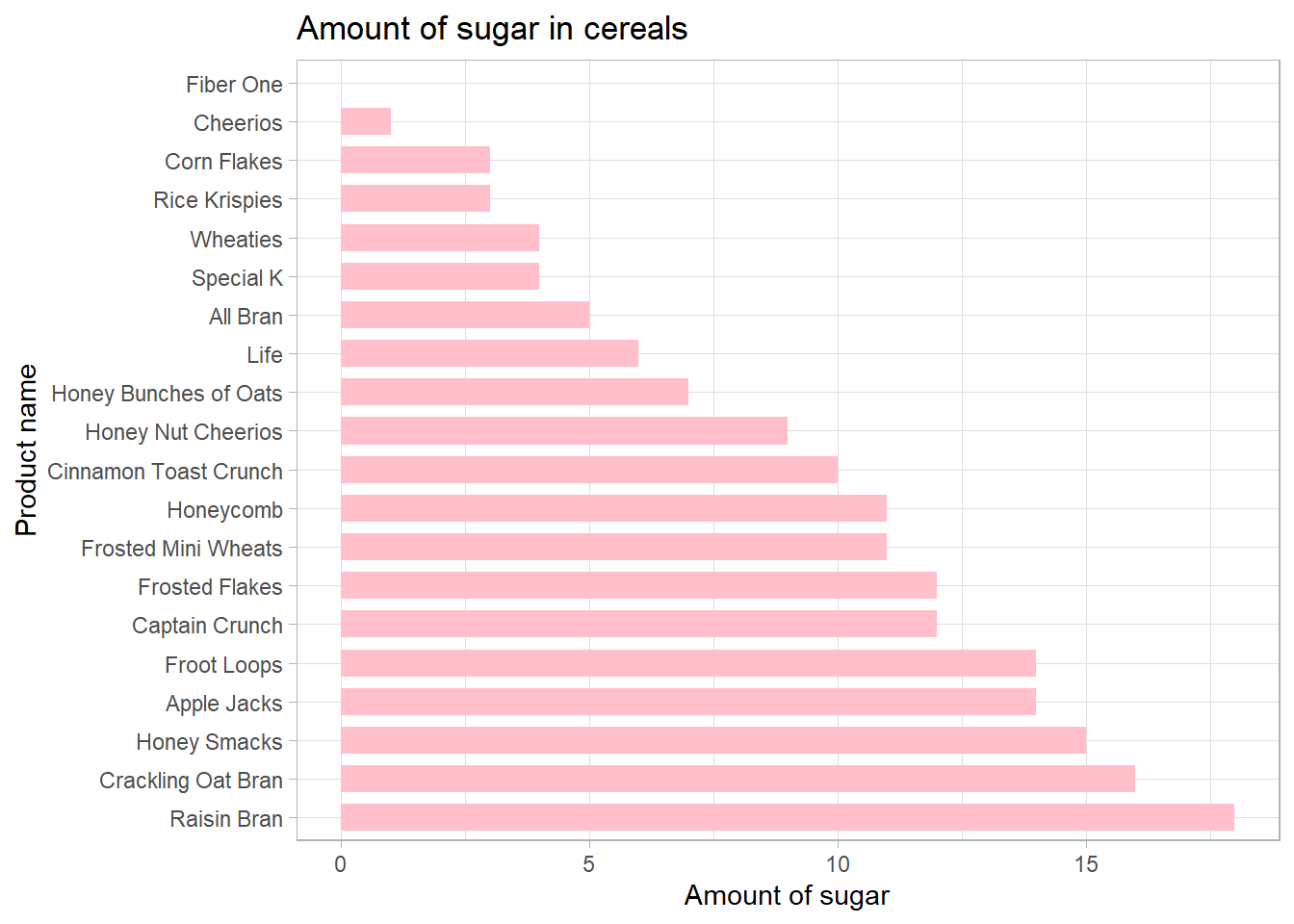

ggplot(cereal, aes(Sugar)) + geom_histogram(bins=12, fill="#69b3a2", color="#e9ecef", alpha=0.9) + xlim(0,20)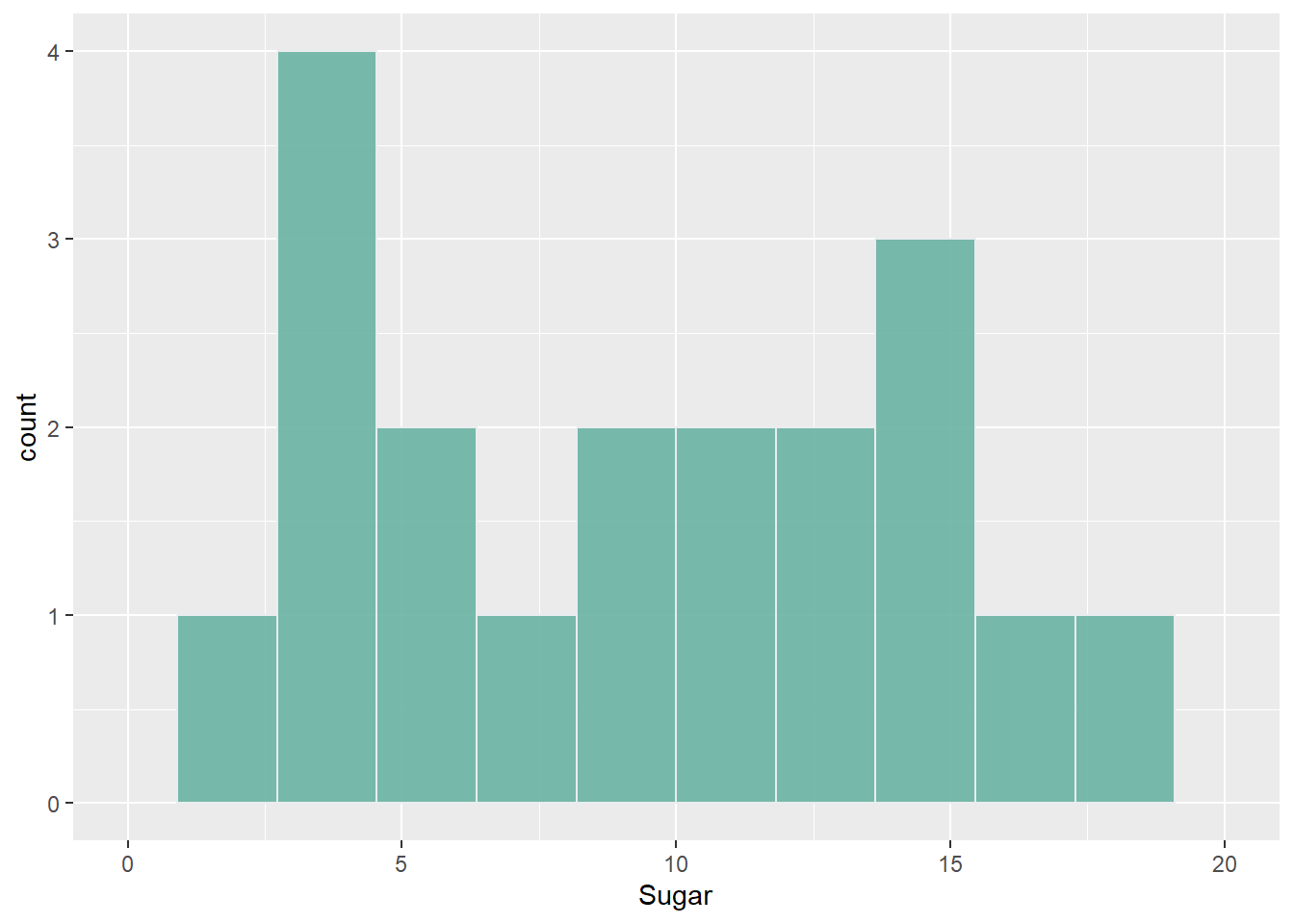

Bivariate Visualization

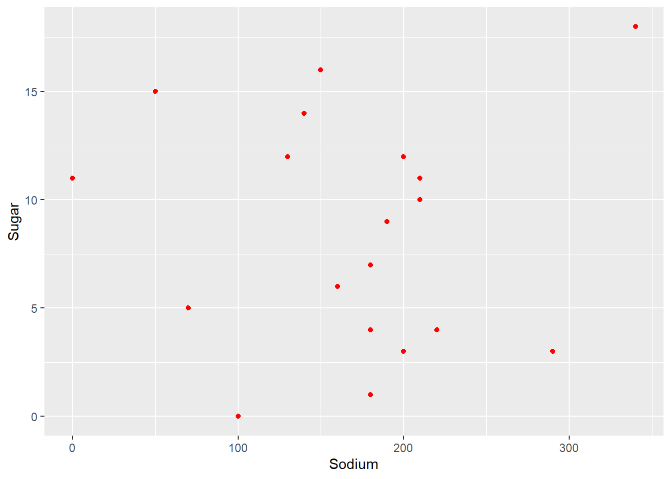
I chose point chart to look if the amount of sugar and sodium somehow corelates.

ggplot(cereal, aes(Sodium, Sugar)) + geom_point (color = "red")