Challenge 5 Instructions

Introduction to Visualization

library(tidyverse)
library(ggplot2)
library(dplyr)
library(summarytools)

knitr::opts_chunk$set(echo = TRUE, warning=FALSE, message=FALSE)

Challenge Overview

Today’s challenge is to:

1. read in a data set, and describe the data set using both words and any supporting information (e.g., tables, etc)
2. tidy data (as needed, including sanity checks)
3. mutate variables as needed (including sanity checks)
4. create at least two univariate visualizations

• try to make them “publication” ready
• Explain why you choose the specific graph type

5. Create at least one bivariate visualization

• try to make them “publication” ready
• Explain why you choose the specific graph type

R Graph Gallery is a good starting point for thinking about what information is conveyed in standard graph types, and includes example R code.

(be sure to only include the category tags for the data you use!)

AB_NYC_2019.csv

Read in data

Using “read_csv” function, I read in AB_NYC_2019.csv as “ab_df”

ab_df = read_csv("_data/AB_NYC_2019.csv")

Briefly describe the data

I explored this dataset to understand how it is structured and what kind of data is included

This dataset consists of 16 columns (variables) and 48895 rows. It includes the follwoing variables.

str(ab_df)

spc_tbl_ [48,895 × 16] (S3: spec_tbl_df/tbl_df/tbl/data.frame)
 $ id                            : num [1:48895] 2539 2595 3647 3831 5022 ...
 $ name                          : chr [1:48895] "Clean & quiet apt home by the park" "Skylit Midtown Castle" "THE VILLAGE OF HARLEM....NEW YORK !" "Cozy Entire Floor of Brownstone" ...
 $ host_id                       : num [1:48895] 2787 2845 4632 4869 7192 ...
 $ host_name                     : chr [1:48895] "John" "Jennifer" "Elisabeth" "LisaRoxanne" ...
 $ neighbourhood_group           : chr [1:48895] "Brooklyn" "Manhattan" "Manhattan" "Brooklyn" ...
 $ neighbourhood                 : chr [1:48895] "Kensington" "Midtown" "Harlem" "Clinton Hill" ...
 $ latitude                      : num [1:48895] 40.6 40.8 40.8 40.7 40.8 ...
 $ longitude                     : num [1:48895] -74 -74 -73.9 -74 -73.9 ...
 $ room_type                     : chr [1:48895] "Private room" "Entire home/apt" "Private room" "Entire home/apt" ...
 $ price                         : num [1:48895] 149 225 150 89 80 200 60 79 79 150 ...
 $ minimum_nights                : num [1:48895] 1 1 3 1 10 3 45 2 2 1 ...
 $ number_of_reviews             : num [1:48895] 9 45 0 270 9 74 49 430 118 160 ...
 $ last_review                   : Date[1:48895], format: "2018-10-19" "2019-05-21" ...
 $ reviews_per_month             : num [1:48895] 0.21 0.38 NA 4.64 0.1 0.59 0.4 3.47 0.99 1.33 ...
 $ calculated_host_listings_count: num [1:48895] 6 2 1 1 1 1 1 1 1 4 ...
 $ availability_365              : num [1:48895] 365 355 365 194 0 129 0 220 0 188 ...
 - attr(*, "spec")=
  .. cols(
  ..   id = col_double(),
  ..   name = col_character(),
  ..   host_id = col_double(),
  ..   host_name = col_character(),
  ..   neighbourhood_group = col_character(),
  ..   neighbourhood = col_character(),
  ..   latitude = col_double(),
  ..   longitude = col_double(),
  ..   room_type = col_character(),
  ..   price = col_double(),
  ..   minimum_nights = col_double(),
  ..   number_of_reviews = col_double(),
  ..   last_review = col_date(format = ""),
  ..   reviews_per_month = col_double(),
  ..   calculated_host_listings_count = col_double(),
  ..   availability_365 = col_double()
  .. )
 - attr(*, "problems")=<externalptr> 

print(summarytools::dfSummary(ab_df,
                         varnumbers = FALSE,
                         plain.ascii  = FALSE,
                         style        = "grid",
                         graph.magnif = 0.80,
                        valid.col    = FALSE),
       method = 'render',
       table.classes = 'table-condensed')

Data Frame Summary

ab_df

Dimensions: 48895 x 16
Duplicates: 0

Variable	Stats / Values	Freqs (% of Valid)	Graph	Missing
id [numeric]	Mean (sd) : 19017143 (10983108) min ≤ med ≤ max: 2539 ≤ 19677284 ≤ 36487245 IQR (CV) : 19680234 (0.6)	48895 distinct values		0 (0.0%)
name [character]	1. Hillside Hotel 2. Home away from home 3. New york Multi-unit build 4. Brooklyn Apartment 5. Loft Suite @ The Box Hous 6. Private Room 7. Artsy Private BR in Fort 8. Private room 9. Beautiful Brooklyn Browns 10. Cozy Brooklyn Apartment [ 47884 others ]	18 ( 0.0% ) 17 ( 0.0% ) 16 ( 0.0% ) 12 ( 0.0% ) 11 ( 0.0% ) 11 ( 0.0% ) 10 ( 0.0% ) 10 ( 0.0% ) 8 ( 0.0% ) 8 ( 0.0% ) 48758 ( 99.8% )		16 (0.0%)
host_id [numeric]	Mean (sd) : 67620011 (78610967) min ≤ med ≤ max: 2438 ≤ 30793816 ≤ 274321313 IQR (CV) : 99612390 (1.2)	37457 distinct values		0 (0.0%)
host_name [character]	1. Michael 2. David 3. Sonder (NYC) 4. John 5. Alex 6. Blueground 7. Sarah 8. Daniel 9. Jessica 10. Maria [ 11442 others ]	417 ( 0.9% ) 403 ( 0.8% ) 327 ( 0.7% ) 294 ( 0.6% ) 279 ( 0.6% ) 232 ( 0.5% ) 227 ( 0.5% ) 226 ( 0.5% ) 205 ( 0.4% ) 204 ( 0.4% ) 46060 ( 94.2% )		21 (0.0%)
neighbourhood_group [character]	1. Bronx 2. Brooklyn 3. Manhattan 4. Queens 5. Staten Island	1091 ( 2.2% ) 20104 ( 41.1% ) 21661 ( 44.3% ) 5666 ( 11.6% ) 373 ( 0.8% )		0 (0.0%)
neighbourhood [character]	1. Williamsburg 2. Bedford-Stuyvesant 3. Harlem 4. Bushwick 5. Upper West Side 6. Hell's Kitchen 7. East Village 8. Upper East Side 9. Crown Heights 10. Midtown [ 211 others ]	3920 ( 8.0% ) 3714 ( 7.6% ) 2658 ( 5.4% ) 2465 ( 5.0% ) 1971 ( 4.0% ) 1958 ( 4.0% ) 1853 ( 3.8% ) 1798 ( 3.7% ) 1564 ( 3.2% ) 1545 ( 3.2% ) 25449 ( 52.0% )		0 (0.0%)
latitude [numeric]	Mean (sd) : 40.7 (0.1) min ≤ med ≤ max: 40.5 ≤ 40.7 ≤ 40.9 IQR (CV) : 0.1 (0)	19048 distinct values		0 (0.0%)
longitude [numeric]	Mean (sd) : -74 (0) min ≤ med ≤ max: -74.2 ≤ -74 ≤ -73.7 IQR (CV) : 0 (0)	14718 distinct values		0 (0.0%)
room_type [character]	1. Entire home/apt 2. Private room 3. Shared room	25409 ( 52.0% ) 22326 ( 45.7% ) 1160 ( 2.4% )		0 (0.0%)
price [numeric]	Mean (sd) : 152.7 (240.2) min ≤ med ≤ max: 0 ≤ 106 ≤ 10000 IQR (CV) : 106 (1.6)	674 distinct values		0 (0.0%)
minimum_nights [numeric]	Mean (sd) : 7 (20.5) min ≤ med ≤ max: 1 ≤ 3 ≤ 1250 IQR (CV) : 4 (2.9)	109 distinct values		0 (0.0%)
number_of_reviews [numeric]	Mean (sd) : 23.3 (44.6) min ≤ med ≤ max: 0 ≤ 5 ≤ 629 IQR (CV) : 23 (1.9)	394 distinct values		0 (0.0%)
last_review [Date]	min : 2011-03-28 med : 2019-05-19 max : 2019-07-08 range : 8y 3m 10d	1764 distinct values		10052 (20.6%)
reviews_per_month [numeric]	Mean (sd) : 1.4 (1.7) min ≤ med ≤ max: 0 ≤ 0.7 ≤ 58.5 IQR (CV) : 1.8 (1.2)	937 distinct values		10052 (20.6%)
calculated_host_listings_count [numeric]	Mean (sd) : 7.1 (33) min ≤ med ≤ max: 1 ≤ 1 ≤ 327 IQR (CV) : 1 (4.6)	47 distinct values		0 (0.0%)
availability_365 [numeric]	Mean (sd) : 112.8 (131.6) min ≤ med ≤ max: 0 ≤ 45 ≤ 365 IQR (CV) : 227 (1.2)	366 distinct values		0 (0.0%)

Generated by summarytools 1.0.1 (R version 4.2.1)
2022-12-20

AB_NYC_2019 documents the information on the accommodation in New York (as you can figure out from the name of the original csv file and the average longitude and latitude) that is registered on Air BnB as of sometime in 2019. The information includes 1) id and name of the accommodation 2) id and name of the host 3) geographic information of the accommodation (neighbourhood_group, latitude, longitude) 4) reservation-related information of the accommodation (room type, price, minimum night per stay) 5) information of the reviews (date of last review, total number of review, average number of review per month) 6) days available of the accommodation per year

The accommodations without any review have NA (missing value) in last_review and reviews_per_month as we can see that the number of missing values in last_review and reviews_per_month (10052) matches the number of accommodations whose number_of_review is 0

ab_df %>% filter(`number_of_reviews` == 0) %>%
  count()

# A tibble: 1 × 1
      n
  <int>
1 10052

Tidy Data

This dataset is quite tidy because one row means one observation (one accommodation), however it can be separated into host_df dataframe and accommodation_df dataframe to make this dataset cleaner and easier to use.

I created accommodation_df as follows removing host_name, calculated_host_listings_count columns. (* We should NOT remove host_id because it will be necessary if we want to join accomodation_df and host_df)

accommodation_df <- ab_df %>%
  select(-c(host_name, calculated_host_listings_count))

head(accommodation_df)

# A tibble: 6 × 14
     id name       host_id neigh…¹ neigh…² latit…³ longi…⁴ room_…⁵ price minim…⁶
  <dbl> <chr>        <dbl> <chr>   <chr>     <dbl>   <dbl> <chr>   <dbl>   <dbl>
1  2539 Clean & q…    2787 Brookl… Kensin…    40.6   -74.0 Privat…   149       1
2  2595 Skylit Mi…    2845 Manhat… Midtown    40.8   -74.0 Entire…   225       1
3  3647 THE VILLA…    4632 Manhat… Harlem     40.8   -73.9 Privat…   150       3
4  3831 Cozy Enti…    4869 Brookl… Clinto…    40.7   -74.0 Entire…    89       1
5  5022 Entire Ap…    7192 Manhat… East H…    40.8   -73.9 Entire…    80      10
6  5099 Large Coz…    7322 Manhat… Murray…    40.7   -74.0 Entire…   200       3
# … with 4 more variables: number_of_reviews <dbl>, last_review <date>,
#   reviews_per_month <dbl>, availability_365 <dbl>, and abbreviated variable
#   names ¹​neighbourhood_group, ²​neighbourhood, ³​latitude, ⁴​longitude,
#   ⁵​room_type, ⁶​minimum_nights

And here is host_df.

host_df <- ab_df %>%
  select(c(host_id, host_name, calculated_host_listings_count))

head(host_df)

# A tibble: 6 × 3
  host_id host_name   calculated_host_listings_count
    <dbl> <chr>                                <dbl>
1    2787 John                                     6
2    2845 Jennifer                                 2
3    4632 Elisabeth                                1
4    4869 LisaRoxanne                              1
5    7192 Laura                                    1
6    7322 Chris                                    1

host_df needs to be cleaned because it has several duplicated information. For example, host_id should be unique however the same host_id appear multiple times as the below table shows.

host_df %>% group_by(host_id) %>%
  count() %>%
  arrange(desc(n))

# A tibble: 37,457 × 2
# Groups:   host_id [37,457]
     host_id     n
       <dbl> <int>
 1 219517861   327
 2 107434423   232
 3  30283594   121
 4 137358866   103
 5  12243051    96
 6  16098958    96
 7  61391963    91
 8  22541573    87
 9 200380610    65
10   1475015    52
# … with 37,447 more rows

So I removed duplicated rows by using distinct() function.

host_df <- host_df %>% distinct(host_id, .keep_all = TRUE) %>%
  arrange(desc(calculated_host_listings_count))

head(host_df)

# A tibble: 6 × 3
    host_id host_name      calculated_host_listings_count
      <dbl> <chr>                                   <dbl>
1 219517861 Sonder (NYC)                              327
2 107434423 Blueground                                232
3  30283594 Kara                                      121
4 137358866 Kazuya                                    103
5  16098958 Jeremy & Laura                             96
6  12243051 Sonder                                     96

Also, I renamed the column name calculated_host_listings_count to make it easier to understand

colnames(host_df)[3] <- "total_accommodation_count"
head(host_df)

# A tibble: 6 × 3
    host_id host_name      total_accommodation_count
      <dbl> <chr>                              <dbl>
1 219517861 Sonder (NYC)                         327
2 107434423 Blueground                           232
3  30283594 Kara                                 121
4 137358866 Kazuya                               103
5  16098958 Jeremy & Laura                        96
6  12243051 Sonder                                96

print(summarytools::dfSummary(host_df,
                         varnumbers = FALSE,
                         plain.ascii  = FALSE,
                         style        = "grid",
                         graph.magnif = 0.80,
                        valid.col    = FALSE),
       method = 'render',
       table.classes = 'table-condensed')

Data Frame Summary

host_df

Dimensions: 37457 x 3
Duplicates: 0

Variable	Stats / Values	Freqs (% of Valid)	Graph	Missing
host_id [numeric]	Mean (sd) : 61445493 (75117502) min ≤ med ≤ max: 2438 ≤ 26790498 ≤ 274321313 IQR (CV) : 81121712 (1.2)	37457 distinct values		0 (0.0%)
host_name [character]	1. Michael 2. David 3. Alex 4. Daniel 5. Sarah 6. John 7. Andrew 8. Chris 9. Maria 10. Anna [ 11442 others ]	335 ( 0.9% ) 318 ( 0.8% ) 226 ( 0.6% ) 208 ( 0.6% ) 199 ( 0.5% ) 188 ( 0.5% ) 163 ( 0.4% ) 162 ( 0.4% ) 161 ( 0.4% ) 156 ( 0.4% ) 35323 ( 94.3% )		18 (0.0%)
total_accommodation_count [numeric]	Mean (sd) : 1.3 (2.8) min ≤ med ≤ max: 1 ≤ 1 ≤ 327 IQR (CV) : 0 (2.1)	47 distinct values		0 (0.0%)

Generated by summarytools 1.0.1 (R version 4.2.1)
2022-12-20

Univariate Visualizations

First, I took a look at the price per night. Most accommodations are concentrated under $600 per night (though still expensive).

ggplot(accommodation_df, aes(price)) + 
  geom_histogram(aes(y= ..density.., binwidth = 20, alpha = 0.5)) +
  geom_density(alpha = 0.5, fill="red")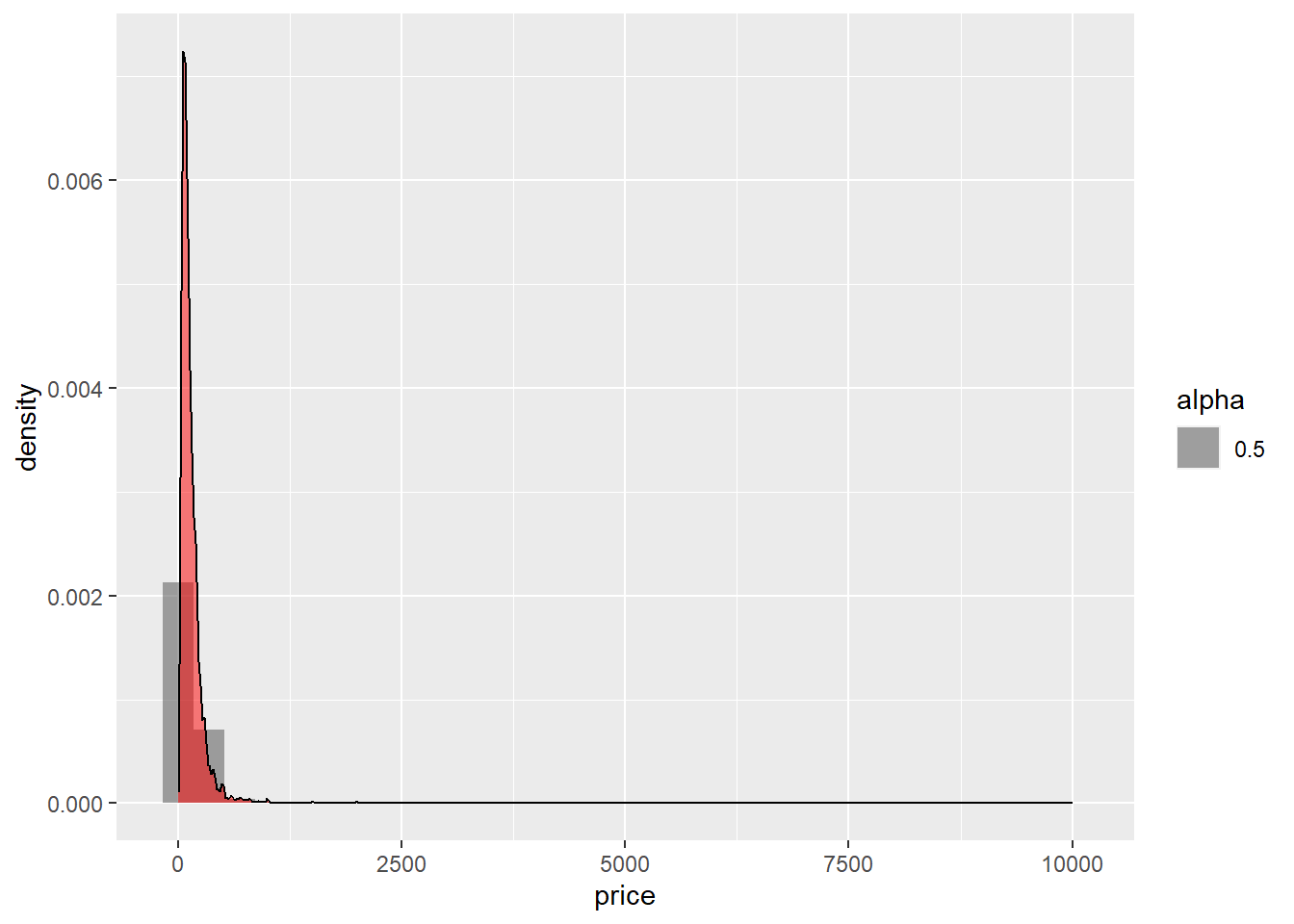

A box-and-whisker diagram shows that there are several Outliers that cost more than USD 2500 per night.

ggplot(accommodation_df, aes(price)) + geom_boxplot()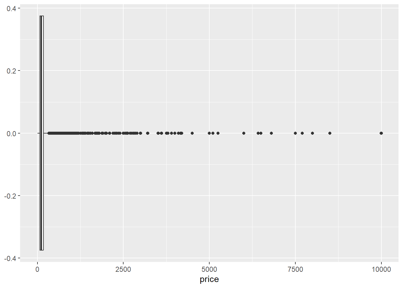

However, it is difficult to see the distribution of smaller values because of some extremely big values so we may need to filter out the accommodation whose price is high, so I decided to analyze only those accommodations whose rates fall between the first (69.0) and third quartiles (175.0)

summary(accommodation_df$price)

   Min. 1st Qu.  Median    Mean 3rd Qu.    Max. 
    0.0    69.0   106.0   152.7   175.0 10000.0 

Bivariate Visualization

ggplot(accommodation_df, aes(price)) + 
  geom_histogram(binwidth = 10) +
  labs(title = "Price per night by room types") +
  theme_bw() +
  facet_wrap(vars(room_type))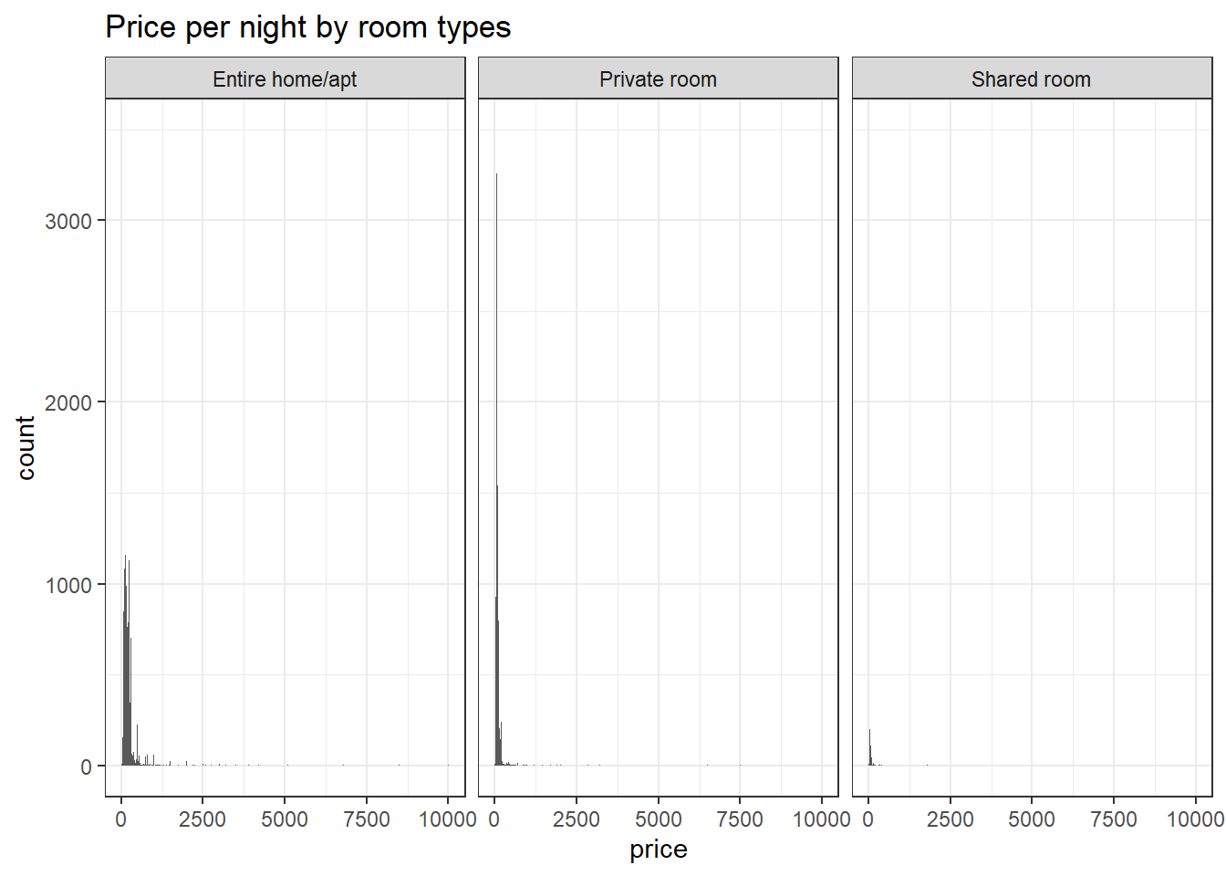

## TRY SCALE PACKAGE

Let’s take a look at the difference in price by room types and neighborhood. (Please note that this data does NOT include accommodation that don’t fall between IQR (69-175 USD)

# Room type 
ggplot(accommodation_df %>% filter(price >= 69 & price<= 175), aes(price)) +
  geom_histogram(binwidth = 10) +
  labs(title = "Price per night by room types") +
  theme_bw() +
  facet_wrap(vars(room_type))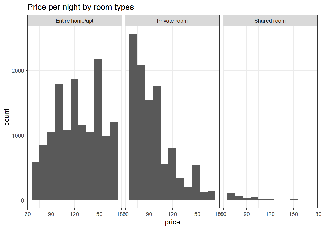

# Neighborhood
ggplot(accommodation_df %>% filter(price >= 69 & price <= 175), aes(price)) +
  geom_histogram() + 
  labs(title = "price per night by neighborhood") + 
  theme_bw() + 
  facet_wrap(vars(neighbourhood_group))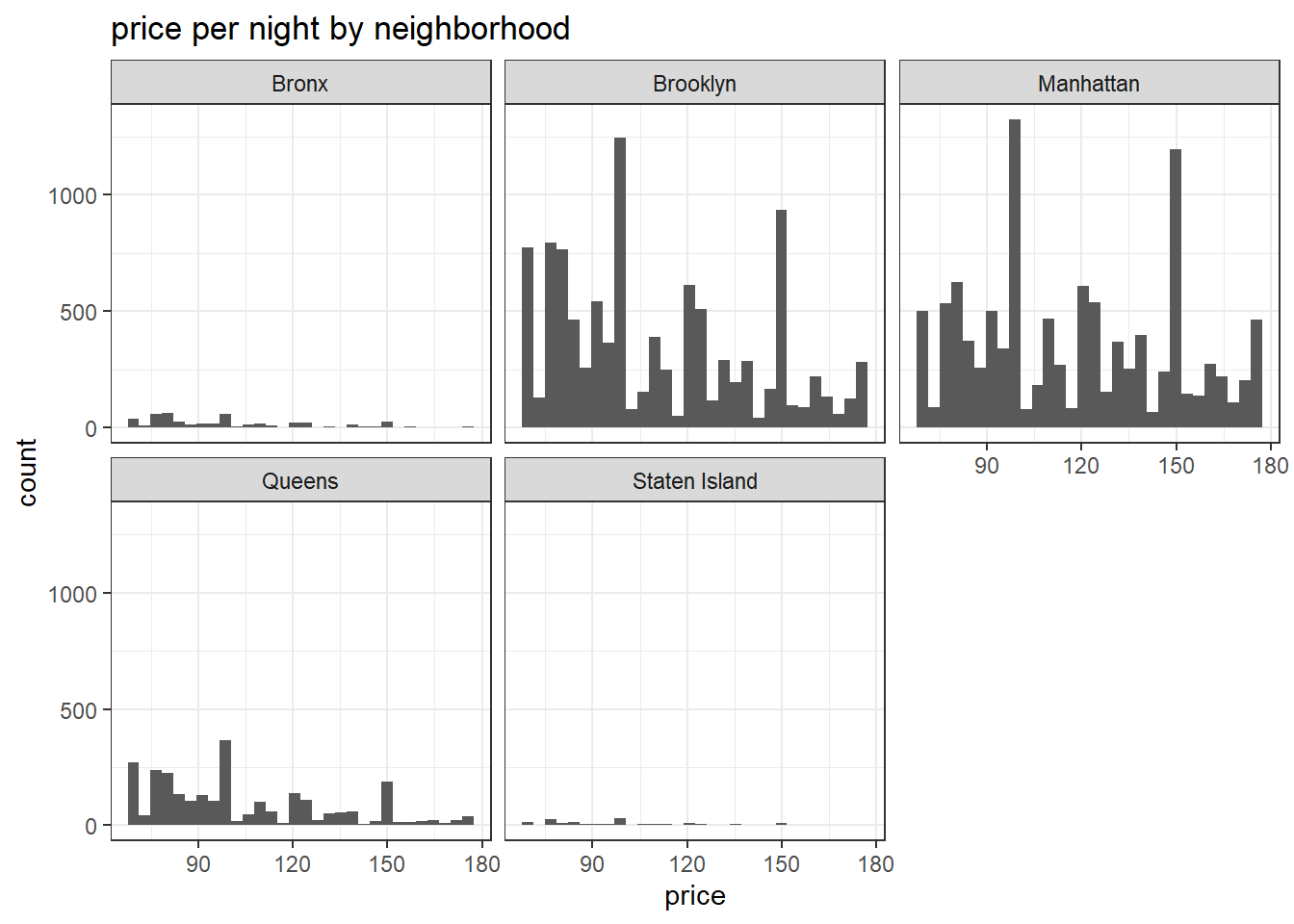

Question!

Since this dataset had some outliers that had a huge value in price and it was hard to visualize the distribution and trend so I decided to use the data that fall within IQR. I don’t know if it was good practice. What is your recommendation?