Challenge 6 Instructions

challenge_6

bechdel_test

movies

Female_Representation

Erika_Nagai

Visualizing Time and Relationships

Author

Erika Nagai

Published

October 23, 2022

library(tidyverse)
library(ggplot2)
library(rjson)
library(jsonlite)
library(summarytools)
library(ggridges)
library(grid)


knitr::opts_chunk$set(echo = TRUE, warning=FALSE, message=FALSE)

Challenge Overview

Today’s challenge is to:

read in a data set, and describe the data set using both words and any supporting information (e.g., tables, etc)
tidy data (as needed, including sanity checks)
mutate variables as needed (including sanity checks)
create at least one graph including time (evolution)

try to make them “publication” ready (optional)
Explain why you choose the specific graph type

Create at least one graph depicting part-whole or flow relationships

try to make them “publication” ready (optional)
Explain why you choose the specific graph type

This week, I chosed to analyze data about female representation in movies, specifically focusing on Bechdel test. According to “Merriam-Webster”, Bechdel test is “a set of criteria used as a test to evaluate a work of fiction (such as a film) on the basis of its inclusion and representation of female characters” (https://www.merriam-webster.com/dictionary/Bechdel%20Test)

It usually includes 1) At least two women are featured 2) These women talk to each other 3) They discuss something other than a man

I used two datasets.

imdb_df: The reviews information taken from IMDb (Internet Movie Database) https://www.imdb.com/interfaces/
bechdel_df: https://bechdeltest.com/api/v1/doc

Read in data

bechdel_df

This data is extracted from bechdeltest API, so I used jsonlite’s read_json function. The values in imdbid are missing “tt” in the beginning and don’t match with the original imdb id so I made a new column new_imdbidthat concatnate “tt” and the value of imdbid

# json_file <- "http://bechdeltest.com/api/v1/getAllMovies"
# bechdel_df <- read_json(path = json_file, simplifyVector = TRUE)
# bechdel_df$titleId <- paste("tt",bechdel_df$imdbid, sep = "")
# 
# 
# head(bechdel_df)

imdb_rating

I downloaded the tsv file compressed in a gz file from this website. https://www.imdb.com/interfaces/ First, I decompressed the gz file by R.usills::gunzip function, and then read in the tsv file.

I do NOT read in the original tsv file in this R Quarto because it is huge and it may cause issues. However, if you want to see what I did to read in the tsv file, you can refer to the below coding.

# I ran the below code to read in a huge gz file. I didn't include this in this quarto file because it doesn't allow me to submit a huge data file and it will cause errors.


# R.utils::gunzip("title.ratings.tsv.gz")
# imdb_rating <- read.delim(file = "title.ratings.tsv", sep = "\t")
# 
# write.csv(imdb_rating, "imdb_rating.csv")

#imdb_rating <- read_csv()

# colnames(imdb_rating)[1] <- "titleId"
# imdb_rating

Then I joined bechdel_df and imdb_rating using titleId and named the new dataset as bechdel_imdb Again, you can see the below code to see how I joined two datasets.

# bechdel_imdb <- left_join(bechdel_df, imdb_rating, by="titleId" )
# 
# write.csv(bechdel_imdb, "~/DACSS/601/601_Fall_2022/posts/_data/bechdel_imdb.csv")
bechdel_imdb <- read_csv("~/DACSS/601/601_Fall_2022/posts/_data/bechdel_imdb.csv")
bechdel_imdb

# A tibble: 9,802 × 9
    ...1 title                 rating  year    id imdbid titleId avera…¹ numVo…²
   <dbl> <chr>                  <dbl> <dbl> <dbl> <chr>  <chr>     <dbl>   <dbl>
 1     1 inazuma eleven: the …      3  1010 10556 17947… tt1794…     6.8     284
 2     2 Passage de Venus           0  1874  9602 31557… tt3155…     6.9    1729
 3     3 La Rosace Magique          0  1877  9804 14495… tt1449…     6       150
 4     4 Sallie Gardner at a …      0  1878  9603 22214… tt2221…     7.4    3101
 5     5 Le singe musicien          0  1878  9806 12592… tt1259…     6.2     258
 6     6 Athlete Swinging a P…      0  1881  9816 78164… tt7816…     5.2     466
 7     7 Buffalo Running            0  1883  9831 54597… tt5459…     6.3    1029
 8     8 L&#39;homme machine        0  1885  9832 85883… tt8588…     5.3     398
 9     9 Man Walking Around t…      0  1887  9614 20752… tt2075…     5.2    1411
10    10 Cockatoo Flying            0  1887  9836 81331… tt8133…     5.3     207
# … with 9,792 more rows, and abbreviated variable names ¹averageRating,
#   ²numVotes

Describe the dataset

As mentioned, bechdel_imdb dataset is made of two different data, (1) Reviews on movies from IMDb (2) Rating of Bechdel test of movies. This data set contains 9802 rows and 8 columns. Each row represents a movie and the below information about each movie is contained:

year: a year when movie was released
id: Bechdeltest.com unique id
rating: Bechdel test rating (0 means no two women, 1 = no talking between women, 2 = talking about a man, 3 means it passes the test)
title: Title of movies
imdbid: IMDb unique id
titleId: IMDb unique id with “tt” in the beginning (this column was used as foreign key when joining the datasets)
average rating: weighted average of all the individual user ratings from IMDb
numVotes: number of votes the title has received

print(summarytools::dfSummary(bechdel_imdb),
      varnumbers = FALSE,
      plain.ascii  = FALSE,
      style        = "grid",
      graph.magnif = 0.80,
      valid.col    = FALSE,
      method = 'render',
      table.classes = 'table-condensed')

Data Frame Summary

bechdel_imdb

Dimensions: 9802 x 9
Duplicates: 0

Variable

Stats / Values

Freqs (% of Valid)

Graph

Missing

...1 [numeric]

Mean (sd) : 4901.5 (2829.7)

min ≤ med ≤ max:

1 ≤ 4901.5 ≤ 9802

IQR (CV) : 4900.5 (0.6)

9802 distinct values

0 (0.0%)

title [character]

1. Cinderella

2. Dracula

3. Little Women

4. Pride and Prejudice

5. Robin Hood

6. Shelter

7. A Star Is Born

8. Alice in Wonderland

9. Anna Karenina

10. Annie

[ 9547 others ]

5	(	0.1%	)
4	(	0.0%	)
4	(	0.0%	)
4	(	0.0%	)
4	(	0.0%	)
4	(	0.0%	)
3	(	0.0%	)
3	(	0.0%	)
3	(	0.0%	)
3	(	0.0%	)
9765	(	99.6%	)

0 (0.0%)

rating [numeric]

Mean (sd) : 2.1 (1.1)

min ≤ med ≤ max:

0 ≤ 3 ≤ 3

IQR (CV) : 2 (0.5)

0	:	1084	(	11.1%	)
1	:	2124	(	21.7%	)
2	:	1000	(	10.2%	)
3	:	5594	(	57.1%	)

0 (0.0%)

year [numeric]

Mean (sd) : 1996.2 (27)

min ≤ med ≤ max:

1010 ≤ 2006 ≤ 2022

IQR (CV) : 25 (0)

142 distinct values

0 (0.0%)

id [numeric]

Mean (sd) : 5224.9 (3052.9)

min ≤ med ≤ max:

1 ≤ 5211.5 ≤ 10641

IQR (CV) : 5233.5 (0.6)

9802 distinct values

0 (0.0%)

imdbid [character]

1. 0035279
2. 0086425
3. 0117056
4. 2043900
5. 2457282
6. 0000001
7. 0000002
8. 0000003
9. 0000004
10. 0000005
[ 9784 others ]

2	(	0.0%	)
2	(	0.0%	)
2	(	0.0%	)
2	(	0.0%	)
2	(	0.0%	)
1	(	0.0%	)
1	(	0.0%	)
1	(	0.0%	)
1	(	0.0%	)
1	(	0.0%	)
9784	(	99.8%	)

3 (0.0%)

titleId [character]

1. tt

2. tt0035279

3. tt0086425

4. tt0117056

5. tt2043900

6. tt2457282

7. tt0000001

8. tt0000002

9. tt0000003

10. tt0000004

[ 9785 others ]

3	(	0.0%	)
2	(	0.0%	)
2	(	0.0%	)
2	(	0.0%	)
2	(	0.0%	)
2	(	0.0%	)
1	(	0.0%	)
1	(	0.0%	)
1	(	0.0%	)
1	(	0.0%	)
9785	(	99.8%	)

0 (0.0%)

averageRating [numeric]

Mean (sd) : 6.6 (1)

min ≤ med ≤ max:

1.2 ≤ 6.7 ≤ 9.4

IQR (CV) : 1.3 (0.2)

81 distinct values

47 (0.5%)

numVotes [numeric]

Mean (sd) : 80886.1 (168621.4)

min ≤ med ≤ max:

5 ≤ 20558 ≤ 2673050

IQR (CV) : 77543 (2.1)

8833 distinct values

47 (0.5%)

Generated by summarytools 1.0.1 (R version 4.2.1)
2022-12-22

Tidy data

There are three different id columns “id”, “imdbid”, and “titleId”. Only one ID column will be enough so I decided to delete “id” and “imdbid”.

Also the column “…1” is not necessary because this colums only shows the row number, thus I removed the column “…1” as well.

bechdel_imdb <- bechdel_imdb %>% select(-c(id, imdbid, ...1))
colnames(bechdel_imdb)

[1] "title"         "rating"        "year"          "titleId"      
[5] "averageRating" "numVotes"

Also I changed the name of columns to make them easier to understand.

colnames(bechdel_imdb) <- c("title", "rating", "year", "titleId", "averageRating", "numVotes")
bechdel_imdb

# A tibble: 9,802 × 6
   title                         rating  year titleId    averageRating numVotes
   <chr>                          <dbl> <dbl> <chr>              <dbl>    <dbl>
 1 inazuma eleven: the movie          3  1010 tt1794796            6.8      284
 2 Passage de Venus                   0  1874 tt3155794            6.9     1729
 3 La Rosace Magique                  0  1877 tt14495706           6        150
 4 Sallie Gardner at a Gallop         0  1878 tt2221420            7.4     3101
 5 Le singe musicien                  0  1878 tt12592084           6.2      258
 6 Athlete Swinging a Pick            0  1881 tt7816420            5.2      466
 7 Buffalo Running                    0  1883 tt5459794            6.3     1029
 8 L&#39;homme machine                0  1885 tt8588366            5.3      398
 9 Man Walking Around the Corner      0  1887 tt2075247            5.2     1411
10 Cockatoo Flying                    0  1887 tt8133192            5.3      207
# … with 9,792 more rows

I realized that the released year of “inazuma eleven: the movie” is 1010, which doesn’t seem correct. According to the information on the internet, this movie was released in 2010, so I manually corrected this information.

bechdel_imdb$year[bechdel_imdb$year==1010] <- 2010

After cleaning the data, the data contains the following information: * year: a year when movie was released * id: Bechdeltest.com unique id * rating: Bechdel test rating (0 means no two women, 1 = no talking between women, 2 = talking about a man, 3 means it passes the test) * title: Title of movies * imdbid: IMDb unique id * titleId: IMDb unique id with “tt” in the beginning (this column was added to join two datasets)Ha * average rating: weighted average of all the individual user ratings from IMDb * numVotes: number of votes the title has received

Visualization

Before analyzing the data, please note that not all movies have the Bechdel test available on http://bechdeltest.com. I’m able to analyze only the movies that have the Bechdel test rating available and the number of these movies is as follows.

vis <- bechdel_imdb %>%
  group_by(year) %>%
  summarize(
    Total_number_of_movie = n()
  )

ggplot(vis, aes(x=year, y=Total_number_of_movie)) + 
  geom_line() +
  labs(title = "The number of movies that have Bechdel test rating available")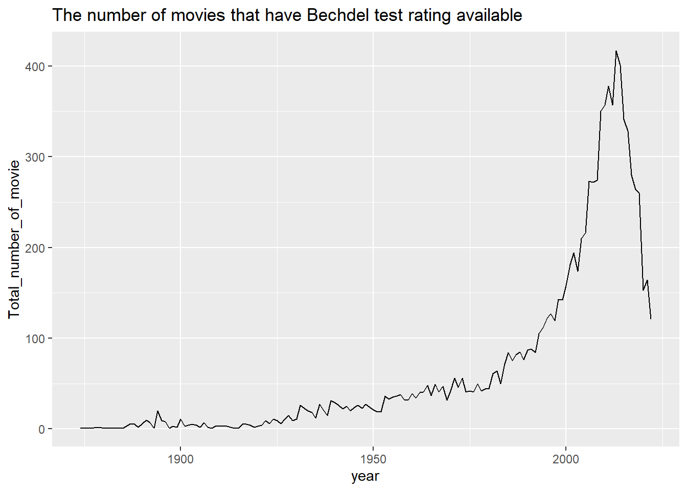

1: Has female representation in movies improved over time?

It seems like the number of movies that pass the Bechdel test is increasing however we cannot see if it’s true because the total number of movies is also increasing.

bechdel_imdb$rating <- as.factor(bechdel_imdb$rating)
vis1 <- bechdel_imdb %>% group_by(year, rating) %>%
  dplyr::summarize(count = n())

ggplot(vis1, aes(x = year, y = count, fill = rating))+
  geom_area()+
  labs(title="Number of movies by Bechdel test rating", y = "Number of movies", x = "Year") +
  scale_fill_discrete(name = "Bechdel Test Rating", labels = c("0: No two women", "1: No women talking each other", "2: Talking about a man", "3: Passes the test"))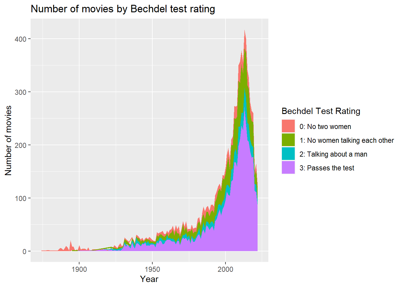

I created the graph of proportion of Bechdel Rating instead of number. This graph shows that the % of movies that pass the Bechdel test is constantly increasing since around 1970. Currently, over 70% of the released movies passes the Bechdel test. Even though most movies feature more than one female, however around 25% of movies still do NOT show two females talking each other.

ggplot(vis1, aes(x = year, y = count, fill = rating))+
  geom_area(position = "fill")+
  labs(title="% of movies by Bechdel test rating", y = "Number of movies", x = "Year") +
  scale_y_continuous(labels = scales::percent)+
  scale_fill_discrete(name = "Bechdel Test Rating", labels = c("0: No two women", "1: No women talking each other", "2: Talking about a man", "3: Passes the test")) +
  annotate("segment", x =1970, xend = 2000, y = 0.35, yend = 0.50, colour = "black", arrow = arrow())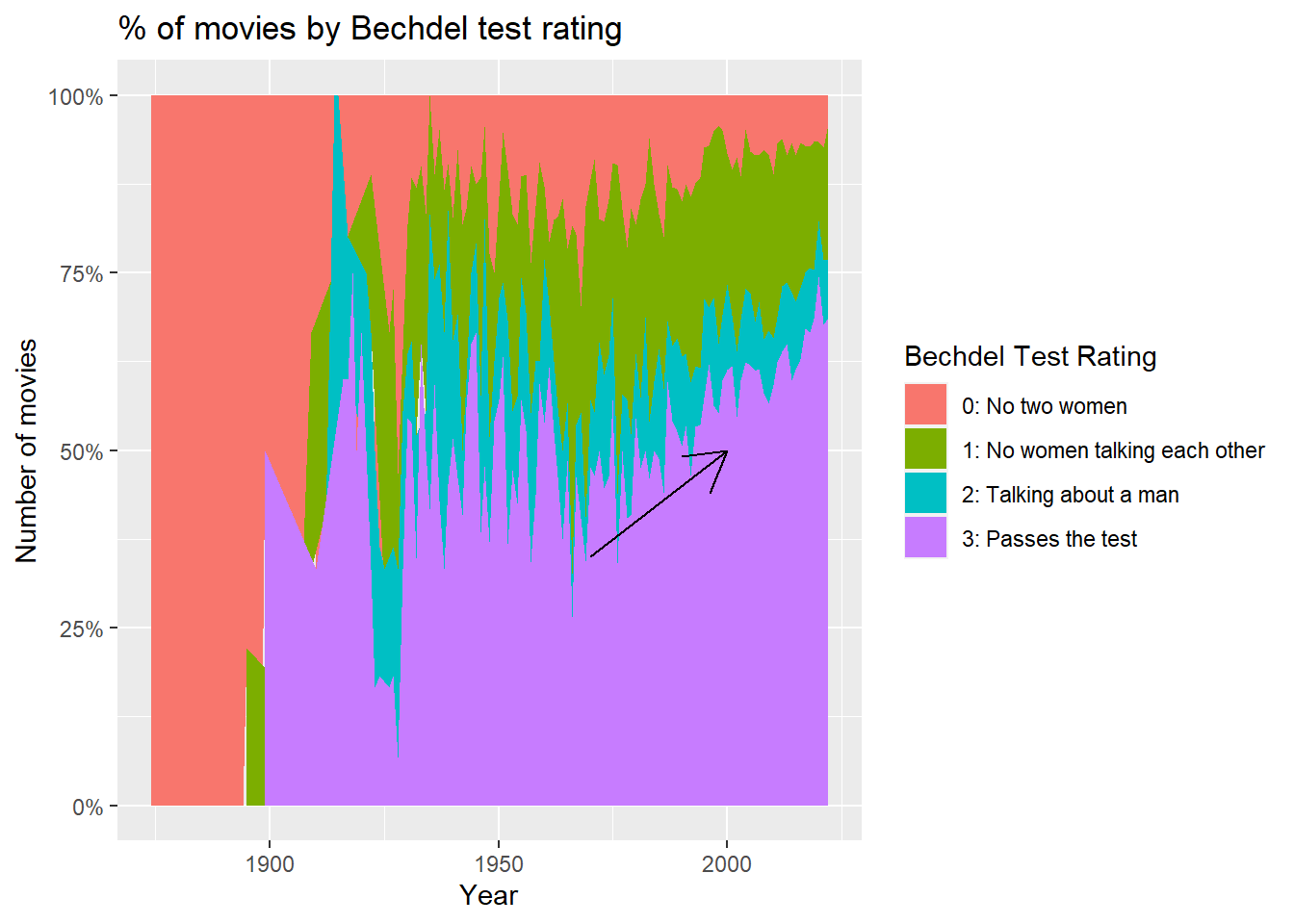

Since there is only a small number of rated movies before 1950, the percentage graph does not appear smooth. I decided to focus on the movies released in 1950 or after.

ggplot(vis1 %>% filter(year >= 1950), aes(x = year, y = count, fill = rating))+
  geom_area(position = "fill")+
  labs(title="% of movies by Bechdel test rating", y = "Number of movies", x = "Year") +
  scale_y_continuous(labels = scales::percent)+
  scale_fill_discrete(name = "Bechdel Test Rating", labels = c("0: No two women", "1: No women talking each other", "2: Talking about a man", "3: Passes the test"))+
  annotate("segment", x =1970, xend = 2000, y = 0.35, yend = 0.50, colour = "black", arrow = arrow())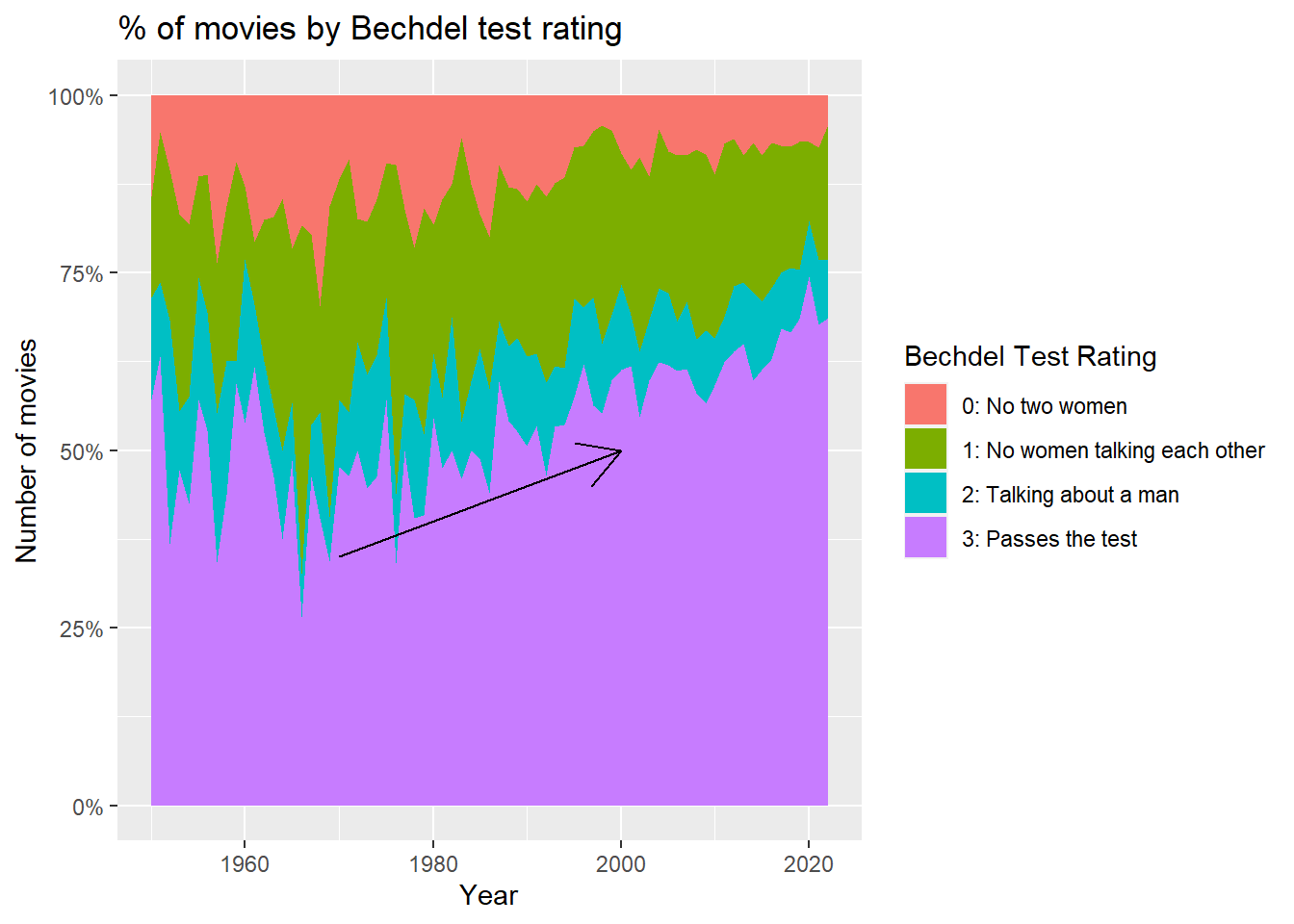

2: Are movies in which women are represented more popular?

If people value female representation in movies, the movies that have a better rating of Bechdel test will score higher on the reviews. However, the below graph doesn’t show such trend clearly.

ggplot(bechdel_imdb %>% filter(year >= 1950), aes(x=year, y=averageRating)) + 
  geom_point(aes(colour=factor(rating))) +
  xlab("Year") +
  ylab("IBDm Review Score") +
  scale_color_discrete(name = "Bechdel Test Rating", labels = c("0: No two women", "1: No women talking each other", "2: Talking about a man", "3: Passes the test"))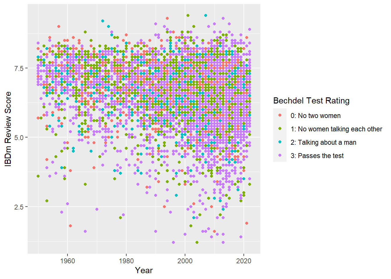

I created a facet graph to see the trend more clearly, however, it seems that the rating of Bechdel test doesn’t affect the review rating.

ggplot(bechdel_imdb %>% filter(year >= 1950), aes(x=year, y=averageRating)) + 
  geom_point() +
  xlab("Year") +
  labs(title = "IMDb review rating by bechdel test rating")+
  ylab("IBDm Review Score") +
  scale_color_discrete(name = "Bechdel Test Rating", labels = c("0: No two women", "1: No women talking each other", "2: Talking about a man", "3: Passes the test")) +
  
  
  facet_wrap(vars(factor(rating)))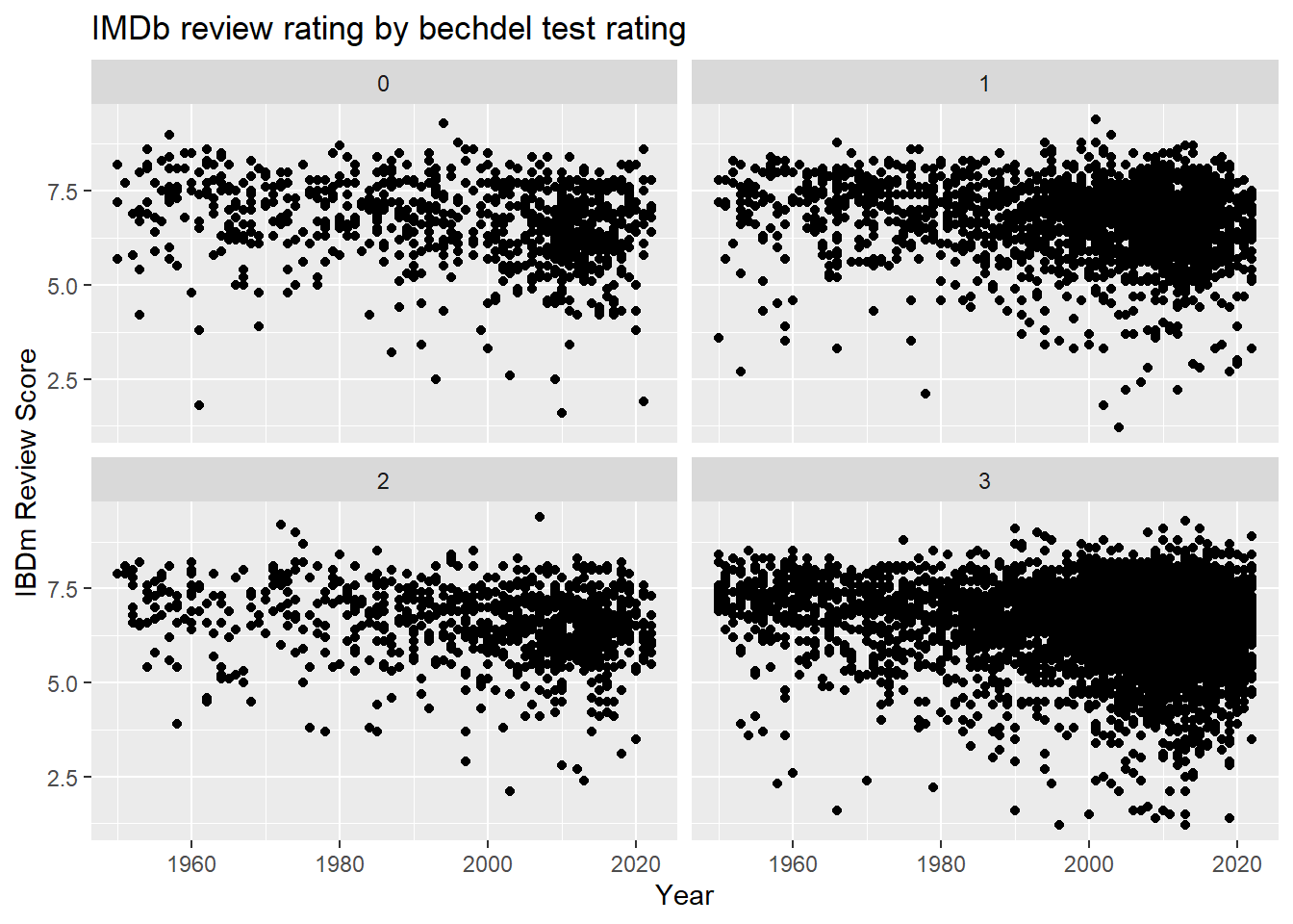

Violin plot or line of average

For further study, I would like to find out: 1) The trend of the number of proportion of the movies that pass Bechdel Test in different regions (Europe, Asia, Middle East, etc) 2) Whether or not a movie passes the Bechdel Test affects the movie’s success (audience and expert reviews, revenue)?