Challenge 6 Instructions

challenge_6

hotel_bookings

air_bnb

fed_rate

debt

usa_households

abc_poll

Visualizing Time and Relationships

Author

Meredith Rolfe

Published

August 23, 2022

library(tidyverse)
library(ggplot2)

knitr::opts_chunk$set(echo = TRUE, warning=FALSE, message=FALSE)

Challenge Overview

Today’s challenge is to:

read in a data set, and describe the data set using both words and any supporting information (e.g., tables, etc)
tidy data (as needed, including sanity checks)
mutate variables as needed (including sanity checks)
create at least one graph including time (evolution)

try to make them “publication” ready (optional)
Explain why you choose the specific graph type

Create at least one graph depicting part-whole or flow relationships

try to make them “publication” ready (optional)
Explain why you choose the specific graph type

R Graph Gallery is a good starting point for thinking about what information is conveyed in standard graph types, and includes example R code.

(be sure to only include the category tags for the data you use!)

Read in data

Read in one (or more) of the following datasets, using the correct R package and command.

debt ⭐
fed_rate ⭐⭐
abc_poll ⭐⭐⭐
usa_hh ⭐⭐⭐
hotel_bookings ⭐⭐⭐⭐
AB_NYC ⭐⭐⭐⭐⭐

ab_nyc <- read_csv("_data/AB_NYC_2019.csv")
ab_nyc

# A tibble: 48,895 × 16
      id name      host_id host_…¹ neigh…² neigh…³ latit…⁴ longi…⁵ room_…⁶ price
   <dbl> <chr>       <dbl> <chr>   <chr>   <chr>     <dbl>   <dbl> <chr>   <dbl>
 1  2539 Clean & …    2787 John    Brookl… Kensin…    40.6   -74.0 Privat…   149
 2  2595 Skylit M…    2845 Jennif… Manhat… Midtown    40.8   -74.0 Entire…   225
 3  3647 THE VILL…    4632 Elisab… Manhat… Harlem     40.8   -73.9 Privat…   150
 4  3831 Cozy Ent…    4869 LisaRo… Brookl… Clinto…    40.7   -74.0 Entire…    89
 5  5022 Entire A…    7192 Laura   Manhat… East H…    40.8   -73.9 Entire…    80
 6  5099 Large Co…    7322 Chris   Manhat… Murray…    40.7   -74.0 Entire…   200
 7  5121 BlissArt…    7356 Garon   Brookl… Bedfor…    40.7   -74.0 Privat…    60
 8  5178 Large Fu…    8967 Shunic… Manhat… Hell's…    40.8   -74.0 Privat…    79
 9  5203 Cozy Cle…    7490 MaryEl… Manhat… Upper …    40.8   -74.0 Privat…    79
10  5238 Cute & C…    7549 Ben     Manhat… Chinat…    40.7   -74.0 Entire…   150
# … with 48,885 more rows, 6 more variables: minimum_nights <dbl>,
#   number_of_reviews <dbl>, last_review <date>, reviews_per_month <dbl>,
#   calculated_host_listings_count <dbl>, availability_365 <dbl>, and
#   abbreviated variable names ¹host_name, ²neighbourhood_group,
#   ³neighbourhood, ⁴latitude, ⁵longitude, ⁶room_type

summary(ab_nyc)

       id               name              host_id           host_name        
 Min.   :    2539   Length:48895       Min.   :     2438   Length:48895      
 1st Qu.: 9471945   Class :character   1st Qu.:  7822033   Class :character  
 Median :19677284   Mode  :character   Median : 30793816   Mode  :character  
 Mean   :19017143                      Mean   : 67620011                     
 3rd Qu.:29152178                      3rd Qu.:107434423                     
 Max.   :36487245                      Max.   :274321313                     
                                                                             
 neighbourhood_group neighbourhood         latitude       longitude     
 Length:48895        Length:48895       Min.   :40.50   Min.   :-74.24  
 Class :character    Class :character   1st Qu.:40.69   1st Qu.:-73.98  
 Mode  :character    Mode  :character   Median :40.72   Median :-73.96  
                                        Mean   :40.73   Mean   :-73.95  
                                        3rd Qu.:40.76   3rd Qu.:-73.94  
                                        Max.   :40.91   Max.   :-73.71  
                                                                        
  room_type             price         minimum_nights    number_of_reviews
 Length:48895       Min.   :    0.0   Min.   :   1.00   Min.   :  0.00   
 Class :character   1st Qu.:   69.0   1st Qu.:   1.00   1st Qu.:  1.00   
 Mode  :character   Median :  106.0   Median :   3.00   Median :  5.00   
                    Mean   :  152.7   Mean   :   7.03   Mean   : 23.27   
                    3rd Qu.:  175.0   3rd Qu.:   5.00   3rd Qu.: 24.00   
                    Max.   :10000.0   Max.   :1250.00   Max.   :629.00   
                                                                         
  last_review         reviews_per_month calculated_host_listings_count
 Min.   :2011-03-28   Min.   : 0.010    Min.   :  1.000               
 1st Qu.:2018-07-08   1st Qu.: 0.190    1st Qu.:  1.000               
 Median :2019-05-19   Median : 0.720    Median :  1.000               
 Mean   :2018-10-04   Mean   : 1.373    Mean   :  7.144               
 3rd Qu.:2019-06-23   3rd Qu.: 2.020    3rd Qu.:  2.000               
 Max.   :2019-07-08   Max.   :58.500    Max.   :327.000               
 NA's   :10052        NA's   :10052                                   
 availability_365
 Min.   :  0.0   
 1st Qu.:  0.0   
 Median : 45.0   
 Mean   :112.8   
 3rd Qu.:227.0   
 Max.   :365.0

Briefly describe the data

I chose to work with the NYC AirBNB data. It consists of 16 variables for 48,895 different AirBNB listings. The variables consist of listing name and ID, host name and ID, neighborhood and neighborhood_group(borough), latitude and longitude, room type, price, min nights, number of reviews, last review, reviews per month, host listings count, and days of availability.

Tidy Data (as needed)

I took a look at the summary statistics for the data on the read in. A quick observation I made was that there were 10052 AirBNBs with no review. This is something that I want to filter out so I can accurately make a graph based on review date.

new_abnyc <- filter(ab_nyc, `number_of_reviews` > 0)
new_abnyc

# A tibble: 38,843 × 16
      id name      host_id host_…¹ neigh…² neigh…³ latit…⁴ longi…⁵ room_…⁶ price
   <dbl> <chr>       <dbl> <chr>   <chr>   <chr>     <dbl>   <dbl> <chr>   <dbl>
 1  2539 Clean & …    2787 John    Brookl… Kensin…    40.6   -74.0 Privat…   149
 2  2595 Skylit M…    2845 Jennif… Manhat… Midtown    40.8   -74.0 Entire…   225
 3  3831 Cozy Ent…    4869 LisaRo… Brookl… Clinto…    40.7   -74.0 Entire…    89
 4  5022 Entire A…    7192 Laura   Manhat… East H…    40.8   -73.9 Entire…    80
 5  5099 Large Co…    7322 Chris   Manhat… Murray…    40.7   -74.0 Entire…   200
 6  5121 BlissArt…    7356 Garon   Brookl… Bedfor…    40.7   -74.0 Privat…    60
 7  5178 Large Fu…    8967 Shunic… Manhat… Hell's…    40.8   -74.0 Privat…    79
 8  5203 Cozy Cle…    7490 MaryEl… Manhat… Upper …    40.8   -74.0 Privat…    79
 9  5238 Cute & C…    7549 Ben     Manhat… Chinat…    40.7   -74.0 Entire…   150
10  5295 Beautifu…    7702 Lena    Manhat… Upper …    40.8   -74.0 Entire…   135
# … with 38,833 more rows, 6 more variables: minimum_nights <dbl>,
#   number_of_reviews <dbl>, last_review <date>, reviews_per_month <dbl>,
#   calculated_host_listings_count <dbl>, availability_365 <dbl>, and
#   abbreviated variable names ¹host_name, ²neighbourhood_group,
#   ³neighbourhood, ⁴latitude, ⁵longitude, ⁶room_type

summary(new_abnyc)

       id               name              host_id           host_name        
 Min.   :    2539   Length:38843       Min.   :     2438   Length:38843      
 1st Qu.: 8720027   Class :character   1st Qu.:  7033824   Class :character  
 Median :18871455   Mode  :character   Median : 28371926   Mode  :character  
 Mean   :18096462                      Mean   : 64239145                     
 3rd Qu.:27554820                      3rd Qu.:101846466                     
 Max.   :36455809                      Max.   :273841667                     
 neighbourhood_group neighbourhood         latitude       longitude     
 Length:38843        Length:38843       Min.   :40.51   Min.   :-74.24  
 Class :character    Class :character   1st Qu.:40.69   1st Qu.:-73.98  
 Mode  :character    Mode  :character   Median :40.72   Median :-73.95  
                                        Mean   :40.73   Mean   :-73.95  
                                        3rd Qu.:40.76   3rd Qu.:-73.94  
                                        Max.   :40.91   Max.   :-73.71  
  room_type             price         minimum_nights     number_of_reviews
 Length:38843       Min.   :    0.0   Min.   :   1.000   Min.   :  1.0    
 Class :character   1st Qu.:   69.0   1st Qu.:   1.000   1st Qu.:  3.0    
 Mode  :character   Median :  101.0   Median :   2.000   Median :  9.0    
                    Mean   :  142.3   Mean   :   5.868   Mean   : 29.3    
                    3rd Qu.:  170.0   3rd Qu.:   4.000   3rd Qu.: 33.0    
                    Max.   :10000.0   Max.   :1250.000   Max.   :629.0    
  last_review         reviews_per_month calculated_host_listings_count
 Min.   :2011-03-28   Min.   : 0.010    Min.   :  1.000               
 1st Qu.:2018-07-08   1st Qu.: 0.190    1st Qu.:  1.000               
 Median :2019-05-19   Median : 0.720    Median :  1.000               
 Mean   :2018-10-04   Mean   : 1.373    Mean   :  5.165               
 3rd Qu.:2019-06-23   3rd Qu.: 2.020    3rd Qu.:  2.000               
 Max.   :2019-07-08   Max.   :58.500    Max.   :327.000               
 availability_365
 Min.   :  0.0   
 1st Qu.:  0.0   
 Median : 55.0   
 Mean   :114.9   
 3rd Qu.:229.0   
 Max.   :365.0

Looking at the newly filtered data, I still see some things that give me questions. The max reviews per month is 58.5, or almost two reviews per day, which seems impossible. There is also a minimum number of nights of 1250 for a listing, also very questionable. Over a quarter of the listings have 0 days of availability and I am not sure if that will affect anything or not.

rev_bym <- new_abnyc%>%
  arrange(desc(`reviews_per_month`))
rev_bym

# A tibble: 38,843 × 16
         id name   host_id host_…¹ neigh…² neigh…³ latit…⁴ longi…⁵ room_…⁶ price
      <dbl> <chr>    <dbl> <chr>   <chr>   <chr>     <dbl>   <dbl> <chr>   <dbl>
 1 32678719 Enjoy…  2.44e8 Row NYC Manhat… Theate…    40.8   -74.0 Privat…   100
 2 32678720 Great…  2.44e8 Row NYC Manhat… Theate…    40.8   -74.0 Privat…   199
 3 30423106 Lou's…  2.28e8 Louann  Queens  Roseda…    40.7   -73.7 Privat…    45
 4 21550302 JFK C…  1.57e8 Nalicia Queens  Spring…    40.7   -73.8 Privat…    80
 5 22176831 JFK 2…  1.57e8 Nalicia Queens  Spring…    40.7   -73.8 Privat…    50
 6 22750161 JFK 3…  1.57e8 Nalicia Queens  Spring…    40.7   -73.8 Privat…    50
 7 16276632 Cozy …  2.64e7 Daniel… Queens  East E…    40.8   -73.9 Privat…    48
 8 18173787 Cute …  2.64e7 Daniel… Queens  East E…    40.8   -73.9 Privat…    48
 9 28826608 “For …  2.17e8 Brent   Queens  Spring…    40.7   -73.8 Entire…    75
10 31249784 Studi…  2.32e8 Lakshm… Queens  Jamaica    40.7   -73.8 Privat…    67
# … with 38,833 more rows, 6 more variables: minimum_nights <dbl>,
#   number_of_reviews <dbl>, last_review <date>, reviews_per_month <dbl>,
#   calculated_host_listings_count <dbl>, availability_365 <dbl>, and
#   abbreviated variable names ¹host_name, ²neighbourhood_group,
#   ³neighbourhood, ⁴latitude, ⁵longitude, ⁶room_type

It appears to be an outlier, but there is nothing out of the ordinary so I will leave it alone.

nights <- new_abnyc%>%
  arrange(desc(`minimum_nights`))
nights

# A tibble: 38,843 × 16
         id name   host_id host_…¹ neigh…² neigh…³ latit…⁴ longi…⁵ room_…⁶ price
      <dbl> <chr>    <dbl> <chr>   <chr>   <chr>     <dbl>   <dbl> <chr>   <dbl>
 1  4204302 Prime…  1.76e7 Genevi… Manhat… Greenw…    40.7   -74.0 Entire…   180
 2 10053943 Histo…  2.70e6 Glenn … Manhat… Harlem     40.8   -73.9 Entire…    99
 3 20990053 Beaut…  1.51e8 Angie   Brookl… Willia…    40.7   -74.0 Privat…    79
 4  5431845 Beaut…  3.68e6 Aliya   Queens  Long I…    40.8   -73.9 Entire…   134
 5  8668115 Zen R…  9.00e6 Laura   Brookl… Crown …    40.7   -73.9 Privat…    50
 6   568684 800sq…  2.80e6 Alessa… Brookl… Bushwi…    40.7   -73.9 Entire…   115
 7   258690 CHELS…  1.36e6 Andrea  Manhat… Chelsea    40.7   -74.0 Entire…   195
 8   271694 Easy,…  1.39e6 James   Manhat… Midtown    40.8   -74.0 Entire…   125
 9   992977 Park …  4.00e6 Shahdi… Brookl… Park S…    40.7   -74.0 Entire…   100
10  2454507 Close…  9.99e6 Andrew  Manhat… Financ…    40.7   -74.0 Entire…   130
# … with 38,833 more rows, 6 more variables: minimum_nights <dbl>,
#   number_of_reviews <dbl>, last_review <date>, reviews_per_month <dbl>,
#   calculated_host_listings_count <dbl>, availability_365 <dbl>, and
#   abbreviated variable names ¹host_name, ²neighbourhood_group,
#   ³neighbourhood, ⁴latitude, ⁵longitude, ⁶room_type

no_av <- filter(new_abnyc, `availability_365` == 0)
no_av

# A tibble: 12,688 × 16
      id name      host_id host_…¹ neigh…² neigh…³ latit…⁴ longi…⁵ room_…⁶ price
   <dbl> <chr>       <dbl> <chr>   <chr>   <chr>     <dbl>   <dbl> <chr>   <dbl>
 1  5022 Entire A…    7192 Laura   Manhat… East H…    40.8   -73.9 Entire…    80
 2  5121 BlissArt…    7356 Garon   Brookl… Bedfor…    40.7   -74.0 Privat…    60
 3  5203 Cozy Cle…    7490 MaryEl… Manhat… Upper …    40.8   -74.0 Privat…    79
 4  6090 West Vil…   11975 Alina   Manhat… West V…    40.7   -74.0 Entire…   120
 5  7801 Sweet an…   21207 Chaya   Brookl… Willia…    40.7   -74.0 Entire…   299
 6 13050 bright a…   50846 Jennif… Brookl… Bedfor…    40.7   -73.9 Entire…   115
 7 16458 Light-fi…   64056 Sara    Brookl… Park S…    40.7   -74.0 Entire…   225
 8 20300 Great Lo…   76627 Pas     Manhat… East V…    40.7   -74.0 Privat…    50
 9 20913 Charming…   79402 Christ… Brookl… Willia…    40.7   -74.0 Entire…   100
10 27883 East Vil…  120223 Jen     Manhat… East V…    40.7   -74.0 Entire…   100
# … with 12,678 more rows, 6 more variables: minimum_nights <dbl>,
#   number_of_reviews <dbl>, last_review <date>, reviews_per_month <dbl>,
#   calculated_host_listings_count <dbl>, availability_365 <dbl>, and
#   abbreviated variable names ¹host_name, ²neighbourhood_group,
#   ³neighbourhood, ⁴latitude, ⁵longitude, ⁶room_type

count(no_av, `room_type` == "Entire home/apt")

# A tibble: 2 × 2
  `room_type == "Entire home/apt"`     n
  <lgl>                            <int>
1 FALSE                             6065
2 TRUE                              6623

There are a few listings with a high amount of minimum nights. Most are entire homes/apartments, so I am guessing that these are just long term living spaces. I also wanted to see if the all the listings with 0 availability for the year meant anything significant. I found out that half of the listings with no availability were Entire home/apt, which is also consistent with a long term living space.

##Are there any variables that require mutation to be usable in your analysis stream? For example, do you need to calculate new values in order to graph them? Can string values be represented numerically? Do you need to turn any variables into factors and reorder for ease of graphics and visualization?

Time Dependent Visualization

My first visualization is to represent the most current review dates in a density chart. I felt like this is the best visual way to represent the reviews over time combined with the quatity of data.

review_dates <- new_abnyc %>%
  ggplot(aes(x = `last_review`)) +
  geom_density(fill="cyan") +
  labs(x="Most Recent Review Date", title = "Density of Latest Review Dates for NYC AirBNB") +
  theme_dark()
review_dates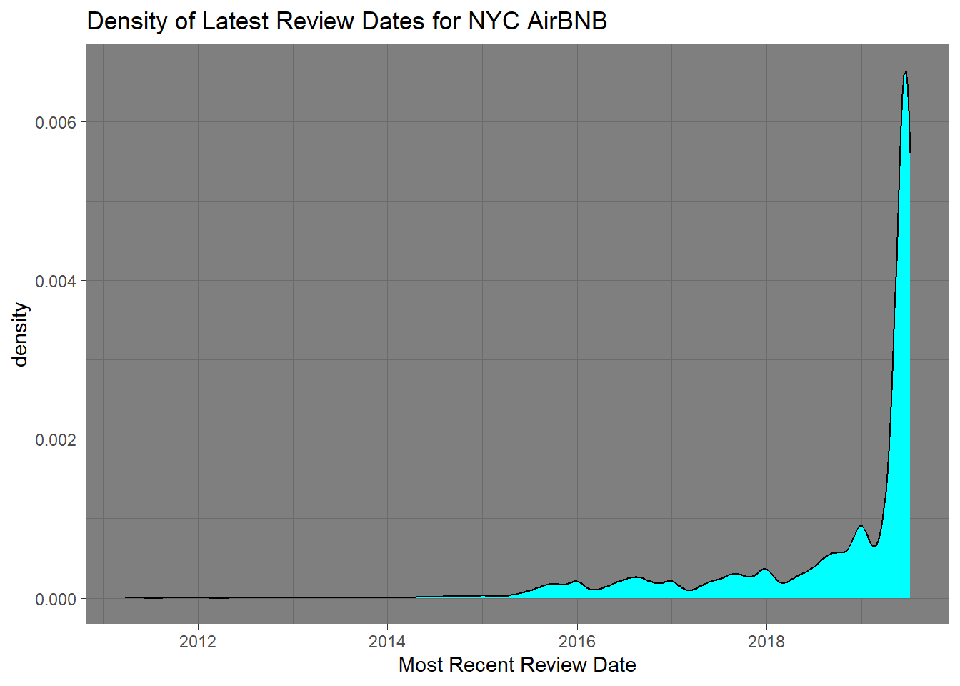

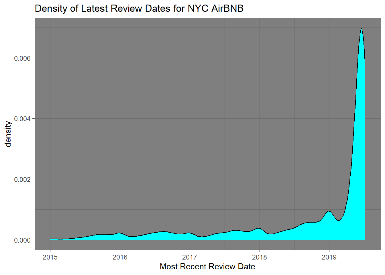
To get a better visual for the data I filtered the data so that it only shows from 2015 onward.

review_dates_2015 <- new_abnyc %>%
  filter(`last_review` >= "2015-01-01")%>%
  ggplot(aes(x = `last_review`)) +
  geom_density(fill="cyan") +
  labs(x="Most Recent Review Date", title = "Density of Latest Review Dates for NYC AirBNB") +
  theme_dark()
review_dates_2015

Challenge Overview

Read in data

Briefly describe the data

Tidy Data (as needed)

Time Dependent Visualization

Visualizing Part-Whole Relationships