library(tidyverse)
library(ggplot2)

knitr::opts_chunk$set(echo = TRUE, warning=FALSE, message=FALSE)Challenge 7
abc_poll
Visualizing Multiple Dimensions
Read in data
- abc_poll ⭐⭐
abc_poll<-read.csv("_data/abc_poll_2021.csv")
library(summarytools)
view(dfSummary(abc_poll))
Error in nchar(xx): invalid multibyte string, element 4Briefly describe the data
The dataframe shows responses to the questionnaire. The respondents are adults (age 18-91) from the USA. - We can see some demographic data like education, income, age, state, etc (column 4-17). - Responses to other questions (about views or experience) are in columns 18-28. Column 2 identifies language of the respondent.
Dataset contains of 527 observations and 31 variables.
Tidy Data (as needed)
- rename and delete certain columns
- simplify information in some columns
#Rename and delete certain columns
abc_poll<-rename(abc_poll, language = xspanish, age =  ppage, education5 = ppeduc5, education = ppeducat, gender = ppgender, ethnicity = ppethm, household_size = pphhsize, income = ppinc7, marital_status = ppmarit5, region = ppreg4, rent = pprent, state = ppstaten, work = PPWORKA, employment = ppemploy)
abc_poll <- select(abc_poll, !contains("complete_status"))

#Simplify information in some columns
abc_poll<-abc_poll %>%
  mutate(education5=case_when(education5 == "Bachelor’s degree" ~ "bachelor",
                              education5 == "High school graduate (high school diploma or the equivalent GED)" ~ "hight_school",
                              education5 == "Master’s degree or above" ~ "master",
                              education5 == "No high school diploma or GED" ~ "no_high_school",
                              education5 == "Some college or Associate degree" ~ "college/associate"))

abc_poll<-abc_poll %>%
  mutate(education=case_when(education == "Bachelors degree or higher" ~ "bachelor",
                              education == "High school" ~ "high_school",
                              education == "Less than high school" ~ "less_high_school",
                              education == "Some college" ~ "college"))

abc_poll <- abc_poll%>%
  mutate(ethnicity = str_remove_all(ethnicity, c(", Non-Hispanic")))
abc_poll <- abc_poll%>%
  mutate(household_size = str_replace_all (household_size, c("6 or more" = "6<")))
abc_poll <- abc_poll%>%
  mutate(income=case_when(income == "Less than $10,000" ~ "1",
                             income == "$10,000 to $24,999" ~ "2",
                             income == "$25,000 to $49,999" ~ "3",
                             income == "$50,000 to $74,999" ~ "4",
                             income == "$75,000 to $99,999" ~ "5",
                             income == "$100,000 to $149,999" ~ "6",
                             income == "$150,000 or more" ~ "7"))

abc_poll <- abc_poll%>%
  mutate(marital_status = str_replace_all(marital_status, c(" " ="_", "m" = "M")))
abc_poll<-abc_poll %>%
  mutate(QPID = fct_recode(QPID, "dem" = "A Democrat",
                                "rep" = "A Republican",
                                "ind" = "An Independent",
                                "skipped" = "Skipped",
                              "other" = "Something else")) %>%
  mutate(QPID = fct_relevel(QPID, "dem", "ind", "rep","other", "skipped"))
Visualization with Multiple Dimensions
I decided to make simple bar chart to show answer to one of the questions and add gender as another dimension. It will show if there are differences between two groups. I am not sure if it is multiple dimensions because the visualization is very simple. But it shows number of responses, type of response and gender.
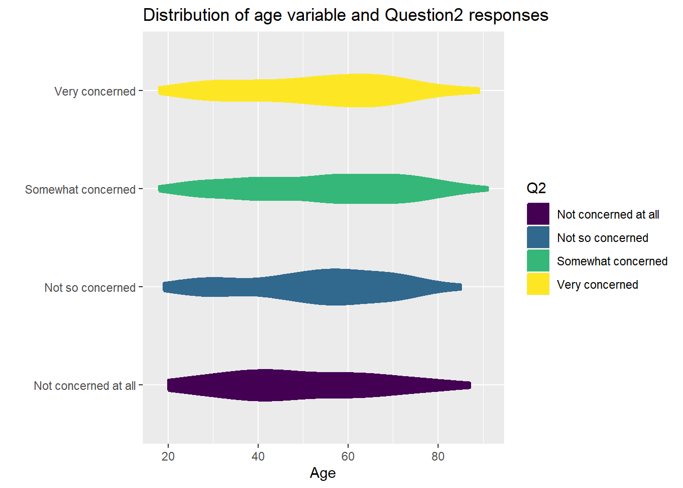
ggplot(abc_poll, aes(Q2, fill=gender)) + geom_bar() + ggtitle("Responses to Question2 by gender") + ggeasy::easy_center_title() + xlab("Question2") + ylab("Responses") + theme(axis.text = element_text(size = 7)) + labs(fill = "Gender")Error in loadNamespace(x): there is no package called 'ggeasy'As a second visualization I chose violin chart to show distribution of age variable for groups who answered Q2 differently.
library(hrbrthemes)
library(viridis)


ggplot(abc_poll, aes(x=Q2, y=age, fill=Q2, color=Q2)) +
    geom_violin(width=0.35, size=1) +
    scale_fill_viridis(discrete=TRUE) +
    scale_color_viridis(discrete=TRUE) +
    coord_flip() + xlab("") +
    ylab("Age") + ggtitle ("Distribution of age variable and Question2 responses")