read in a data set, and describe the data set using both words and any supporting information (e.g., tables, etc)
tidy data (as needed, including sanity checks)
mutate variables as needed (including sanity checks)
Recreate at least two graphs from previous exercises, but introduce at least one additional dimension that you omitted before using ggplot functionality (color, shape, line, facet, etc) The goal is not to create unneeded chart ink (Tufte), but to concisely capture variation in additional dimensions that were collapsed in your earlier 2 or 3 dimensional graphs.
Explain why you choose the specific graph type
If you haven’t tried in previous weeks, work this week to make your graphs “publication” ready with titles, captions, and pretty axis labels and other viewer-friendly features
R Graph Gallery is a good starting point for thinking about what information is conveyed in standard graph types, and includes example R code. And anyone not familiar with Edward Tufte should check out his fantastic books and courses on data visualizaton.
(be sure to only include the category tags for the data you use!)
Read in data
Read in one (or more) of the following datasets, using the correct R package and command.
eggs ⭐
abc_poll ⭐⭐
australian_marriage ⭐⭐
hotel_bookings ⭐⭐⭐
air_bnb ⭐⭐⭐
us_hh ⭐⭐⭐⭐
faostat ⭐⭐⭐⭐⭐
Using read_csv function, I read in AB_NYC_2019.csv as “ab_df”
ab_df =read_csv("_data/AB_NYC_2019.csv")
Briefly describe the data
I explored this dataset to understand how it is structured and what kind of data is included
This dataset consists of 16 columns (variables) and 48895 rows. It includes the follwoing variables.
Generated by summarytools 1.0.1 (R version 4.2.1) 2022-12-20
AB_NYC_2019 documents the information on the accommodation in New York (as you can figure out from the name of the original csv file and the average longitude and latitude) that is registered on Air BnB as of sometime in 2019. The information includes 1) id and name of the accommodation 2) id and name of the host 3) geographic information of the accommodation (neighbourhood_group, latitude, longitude) 4) reservation-related information of the accommodation (room type, price, minimum night per stay) 5) information of the reviews (date of last review, total number of review, average number of review per month) 6) days available of the accommodation per year
The accommodations without any review have NA (missing value) in last_review and reviews_per_month as we can see that the number of missing values in last_review and reviews_per_month (10052) matches the number of accommodations whose number_of_review is 0
This dataset is quite tidy because one row means one observation (one accommodation), however it can be separated into host_df dataframe and accommodation_df dataframe to make this dataset cleaner and easier to use.
###Accommodation_df
I created accommodation_df as follows removing host_name, calculated_host_listings_count columns. (* We should NOT remove host_id because it will be necessary if we want to join accomodation_df and host_df)
I realized that there are 17,541 observations with 0 as price and/or availability_365, which doesn’t make sense for an accommodation listing on AirBnB.
summary(accommodation_df)
       id               name              host_id          neighbourhood_group
 Min.   :    2539   Length:48895       Min.   :     2438   Length:48895
 1st Qu.: 9471945   Class :character   1st Qu.:  7822033   Class :character
 Median :19677284   Mode  :character   Median : 30793816   Mode  :character
 Mean   :19017143                      Mean   : 67620011
 3rd Qu.:29152178                      3rd Qu.:107434423
 Max.   :36487245                      Max.   :274321313

 neighbourhood         latitude       longitude       room_type
 Length:48895       Min.   :40.50   Min.   :-74.24   Length:48895
 Class :character   1st Qu.:40.69   1st Qu.:-73.98   Class :character
 Mode  :character   Median :40.72   Median :-73.96   Mode  :character
                    Mean   :40.73   Mean   :-73.95
                    3rd Qu.:40.76   3rd Qu.:-73.94
                    Max.   :40.91   Max.   :-73.71

     price         minimum_nights    number_of_reviews  last_review
 Min.   :    0.0   Min.   :   1.00   Min.   :  0.00    Min.   :2011-03-28
 1st Qu.:   69.0   1st Qu.:   1.00   1st Qu.:  1.00    1st Qu.:2018-07-08
 Median :  106.0   Median :   3.00   Median :  5.00    Median :2019-05-19
 Mean   :  152.7   Mean   :   7.03   Mean   : 23.27    Mean   :2018-10-04
 3rd Qu.:  175.0   3rd Qu.:   5.00   3rd Qu.: 24.00    3rd Qu.:2019-06-23
 Max.   :10000.0   Max.   :1250.00   Max.   :629.00    Max.   :2019-07-08
                                                       NA's   :10052
 reviews_per_month availability_365
 Min.   : 0.010    Min.   :  0.0
 1st Qu.: 0.190    1st Qu.:  0.0
 Median : 0.720    Median : 45.0
 Mean   : 1.373    Mean   :112.8
 3rd Qu.: 2.020    3rd Qu.:227.0
 Max.   :58.500    Max.   :365.0
 NA's   :10052
# A tibble: 17,541 × 3
   name                                               price availability_365
   <chr>                                              <dbl>            <dbl>
 1 Entire Apt: Spacious Studio/Loft by central park      80                0
 2 BlissArtsSpace!                                       60                0
 3 Cozy Clean Guest Room - Family Apt                    79                0
 4 West Village Nest - Superhost                        120                0
 5 Sweet and Spacious Brooklyn Loft                     299                0
 6 Magnifique Suite au N de Manhattan - vue Cloitres     80                0
 7 bright and stylish duplex                            115                0
 8 Light-filled 2B duplex in the heart of Park Slope!   225                0
 9 Great Location for NYC                                50                0
10 Charming 1 bed GR8 WBurg LOCATION!                   100                0
# … with 17,531 more rows
These listings should be considered unavailable or at least not ready for receiving the travelers, so I created a new column outlier (1 = outlier, 0 = no outlier).
Looking at minimum_nights, I noticed that some accommodations require a lot of days for the minimum nights.
I learned from the below table that 1) The minimum nights of 85% + listings are 7 nights or less. 2) The minimum nights of 98% + listings are 31 nights or less. 3) There are small peaks at 30 nights (3760), 60 nights (106), 90 nights (104), and 120 nights (28), inferring that some listings require 1,2,3, or 4 month stay.
Thus, it is fairly safe to consider that the accommodation that require more than 31 days (1 month) for the minimum nights as outliers. Since these accommodations are not available for short-term travelers, I consider them as “outlier” (outlier = 1)
Some accommodations cost more than 1000 USD per night, which is extremely expensive. Looking at the below table, only less than 0.5% of accommodations charge 1000+ USD per night so I decided to consider those accommodations as outliers.
# A tibble: 6 × 3
  host_id host_name   calculated_host_listings_count
    <dbl> <chr>                                <dbl>
1    2787 John                                     6
2    2845 Jennifer                                 2
3    4632 Elisabeth                                1
4    4869 LisaRoxanne                              1
5    7192 Laura                                    1
6    7322 Chris                                    1
host_df needs to be cleaned because it has several duplicated information. For example, host_id should be unique however the same host_id appear multiple times as the below table shows.
Generated by summarytools 1.0.1 (R version 4.2.1) 2022-12-20
Visualization with Multiple Dimensions
What are the characteristics of each neighborhood?
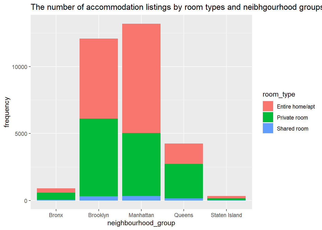
First, I decided to visualize the number of accommodation listings by room types and neighborhood groups.
Most listings are located in Manhattan or Brooklyn.
There are few listings of shared rooms compared to entire home and private rooms.
accommodation_df %>%filter(outlier==0) %>%group_by(neighbourhood_group, room_type)%>% dplyr::summarize(frequency =n() ) %>%ggplot(aes(fill=room_type, y=frequency, x=neighbourhood_group)) +geom_bar(position="stack", stat="identity") +labs(title ="The number of accommodation listings by room types and neibhgourhood groups")
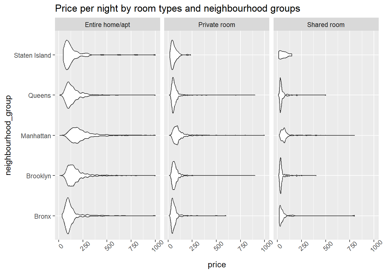
I decided to visualize the price data by neighbourhood group with a violin plot because it allows us to see the distribution and the volume for several groups.
I learned that, 1) Manhattan is the most expensive neighbourhood regardless of room types. 2) Even though Manhattan and Brooklyn are typically more expensive than other neighbourhoods, they offer more reasonable entire home/apartments as well.
accommodation_df %>%filter(outlier==0) %>%ggplot(aes(neighbourhood_group, price)) +geom_violin() +facet_wrap(vars(room_type)) +theme(axis.text.x =element_text(angle =45)) +labs(title ="Price per night by room types and neighbourhood groups") +coord_flip()
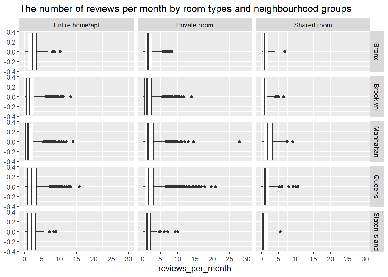
accommodation_df %>%filter(outlier ==0) %>%ggplot(aes(reviews_per_month)) +geom_boxplot() +facet_grid(neighbourhood_group~room_type) +scale_x_continuous(limits=c(0,30), breaks=seq(0,30,5)) +labs(title ="The number of reviews per month by room types and neighbourhood groups")
Source Code
---title: "Challenge 7 Erika Nagai"author: "Erika Nagai"description: "Visualizing Multiple Dimensions"date: "10/31/2022"format: html: toc: true code-copy: true code-tools: truecategories: - challenge_7 - air_bnbeditor: markdown: wrap: sentence---```{r}#| warning: false#| message: falselibrary(tidyverse)library(ggplot2)library(summarytools)library(knitr)library(wordcloud)library(ggwordcloud)knitr::opts_chunk$set(echo =TRUE, warning=FALSE, message=FALSE)```## Challenge OverviewToday's challenge is to:1) read in a data set, and describe the data set using both words and any supporting information (e.g., tables, etc)2) tidy data (as needed, including sanity checks)3) mutate variables as needed (including sanity checks)4) Recreate at least two graphs from previous exercises, but introduce at least one additional dimension that you omitted before using ggplot functionality (color, shape, line, facet, etc) The goal is not to create unneeded [chart ink (Tufte)](https://www.edwardtufte.com/tufte/), but to concisely capture variation in additional dimensions that were collapsed in your earlier 2 or 3 dimensional graphs.- Explain why you choose the specific graph type5) If you haven't tried in previous weeks, work this week to make your graphs "publication" ready with titles, captions, and pretty axis labels and other viewer-friendly features[R Graph Gallery](https://r-graph-gallery.com/) is a good starting point for thinking about what information is conveyed in standard graph types, and includes example R code.And anyone not familiar with Edward Tufte should check out his [fantastic books](https://www.edwardtufte.com/tufte/books_vdqi) and [courses on data visualizaton.](https://www.edwardtufte.com/tufte/courses)(be sure to only include the category tags for the data you use!)## Read in dataRead in one (or more) of the following datasets, using the correct R package and command.- eggs ⭐- abc_poll ⭐⭐- australian_marriage ⭐⭐- hotel_bookings ⭐⭐⭐- air_bnb ⭐⭐⭐- us_hh ⭐⭐⭐⭐- faostat ⭐⭐⭐⭐⭐Using `read_csv` function, I read in AB_NYC_2019.csv as "ab_df"```{r}ab_df =read_csv("_data/AB_NYC_2019.csv")```### Briefly describe the dataI explored this dataset to understand how it is structured and what kind of data is includedThis dataset consists of 16 columns (variables) and 48895 rows.It includes the follwoing variables.```{r}str(ab_df)``````{r}print(summarytools::dfSummary(ab_df,varnumbers =FALSE,plain.ascii =FALSE,style ="grid",graph.magnif =0.80,valid.col =FALSE),method ='render',table.classes ='table-condensed')````AB_NYC_2019` documents the information on the accommodation in New York (as you can figure out from the name of the original csv file and the average longitude and latitude) that is registered on Air BnB as of sometime in 2019.The information includes 1) id and name of the accommodation 2) id and name of the host 3) geographic information of the accommodation (neighbourhood_group, latitude, longitude) 4) reservation-related information of the accommodation (room type, price, minimum night per stay) 5) information of the reviews (date of last review, total number of review, average number of review per month) 6) days available of the accommodation per yearThe accommodations without any review have NA (missing value) in `last_review` and `reviews_per_month` as we can see that the number of missing values in `last_review` and `reviews_per_month` (10052) matches the number of accommodations whose `number_of_review` is 0```{r}ab_df %>%filter(`number_of_reviews`==0) %>%count()```This dataset is quite tidy because one row means one observation (one accommodation), however it can be separated into `host_df` dataframe and `accommodation_df` dataframe to make this dataset cleaner and easier to use.\###`Accommodation_df`I created `accommodation_df` as follows removing `host_name`, `calculated_host_listings_count` columns.(\* We should NOT remove `host_id` because it will be necessary if we want to join `accomodation_df` and `host_df`)```{r}accommodation_df <- ab_df %>%select(-c(host_name, calculated_host_listings_count))head(accommodation_df)```I realized that there are 17,541 observations with 0 as `price` and/or `availability_365`, which doesn't make sense for an accommodation listing on AirBnB.```{r}summary(accommodation_df)accommodation_df %>%select(c("name", "price", "availability_365")) %>%filter(price ==0| availability_365 ==0)```These listings should be considered unavailable or at least not ready for receiving the travelers, so I created a new column `outlier` (1 = outlier, 0 = no outlier).```{r}accommodation_df <- accommodation_df %>%mutate(outlier =case_when(.$price ==0|.$availability_365 ==0~1, TRUE~0))```Looking at `minimum_nights`, I noticed that some accommodations require a lot of days for the minimum nights.I learned from the below table that 1) The minimum nights of 85% + listings are 7 nights or less.2) The minimum nights of 98% + listings are 31 nights or less.3) There are small peaks at 30 nights (3760), 60 nights (106), 90 nights (104), and 120 nights (28), inferring that some listings require 1,2,3, or 4 month stay.```{r}accommodation_df %>%group_by(minimum_nights) %>% dplyr::summarize(frequency =n(), ) %>%mutate(cumulative_percentage =cumsum(frequency)/sum(frequency)*100 ) %>%kable()```Thus, it is fairly safe to consider that the accommodation that require more than 31 days (1 month) for the minimum nights as outliers.Since these accommodations are not available for short-term travelers, I consider them as "outlier" (`outlier` = 1)```{r}accommodation_df <- accommodation_df %>%mutate(outlier =case_when(.$price ==0|.$availability_365 ==0| minimum_nights >31~1, TRUE~0))accommodation_df```Some accommodations cost more than 1000 USD per night, which is extremely expensive.Looking at the below table, only less than 0.5% of accommodations charge 1000+ USD per night so I decided to consider those accommodations as outliers.```{r}accommodation_df %>%group_by(price) %>% dplyr::summarize(frequency =n(), ) %>%mutate(cumulative_percentage =cumsum(frequency)/sum(frequency)*100 ) %>%kable()``````{r}accommodation_df <- accommodation_df %>%mutate(outlier =case_when(.$price ==0|.$price >1000|.$availability_365 ==0| minimum_nights >31~1, TRUE~0))accommodation_df```\###`host_df`.```{r}host_df <- ab_df %>%select(c(host_id, host_name, calculated_host_listings_count))head(host_df)````host_df` needs to be cleaned because it has several duplicated information.For example, `host_id` should be unique however the same host_id appear multiple times as the below table shows.```{r}host_df %>%group_by(host_id) %>% dplyr::summarise(number =n()) %>%arrange(desc(number))```So I removed duplicated rows by using `distinct()` function```{r}host_df <- host_df %>%distinct(host_id, .keep_all =TRUE) %>%arrange(desc(calculated_host_listings_count))head(host_df)```Also, I renamed the column name `calculated_host_listings_count` to make it easier to understand```{r}colnames(host_df)[3] <-"total_accommodation_count"head(host_df)``````{r}print(summarytools::dfSummary(host_df,varnumbers =FALSE,plain.ascii =FALSE,style ="grid",graph.magnif =0.80,valid.col =FALSE),method ='render',table.classes ='table-condensed')```## Visualization with Multiple Dimensions**What are the characteristics of each neighborhood?**First, I decided to visualize the number of accommodation listings by room types and neighborhood groups.1) Most listings are located in Manhattan or Brooklyn.2) There are few listings of shared rooms compared to entire home and private rooms.```{r}accommodation_df %>%filter(outlier==0) %>%group_by(neighbourhood_group, room_type)%>% dplyr::summarize(frequency =n() ) %>%ggplot(aes(fill=room_type, y=frequency, x=neighbourhood_group)) +geom_bar(position="stack", stat="identity") +labs(title ="The number of accommodation listings by room types and neibhgourhood groups")```I decided to visualize the price data by neighbourhood group with a violin plot because it allows us to see the distribution and the volume for several groups.I learned that, 1) Manhattan is the most expensive neighbourhood regardless of room types.2) Even though Manhattan and Brooklyn are typically more expensive than other neighbourhoods, they offer more reasonable entire home/apartments as well.```{r}accommodation_df %>%filter(outlier==0) %>%ggplot(aes(neighbourhood_group, price)) +geom_violin() +facet_wrap(vars(room_type)) +theme(axis.text.x =element_text(angle =45)) +labs(title ="Price per night by room types and neighbourhood groups") +coord_flip()``````{r}accommodation_df %>%filter(outlier ==0) %>%ggplot(aes(reviews_per_month)) +geom_boxplot() +facet_grid(neighbourhood_group~room_type) +scale_x_continuous(limits=c(0,30), breaks=seq(0,30,5)) +labs(title ="The number of reviews per month by room types and neighbourhood groups")```