Challenge 8 Guanhua Tan

challenge_8

pisa2018

Joining Data

Author

Guanhua Tan

Published

November 10, 2022

library(tidyverse)
library(ggplot2)
install.packages("tmap")

Error in contrib.url(repos, "source"): trying to use CRAN without setting a mirror

library(tmap)
library(dplyr)

knitr::opts_chunk$set(echo = TRUE, warning=FALSE, message=FALSE)

Challenge Overview

Today’s challenge is to:

read in multiple data sets, and describe the data set using both words and any supporting information (e.g., tables, etc)
tidy data (as needed, including sanity checks)
mutate variables as needed (including sanity checks)
join two or more data sets and analyze some aspect of the joined data

(be sure to only include the category tags for the data you use!)

Read in data

Read in one (or more) of the following datasets, using the correct R package and command.

Pisa2018

# read the data
pisa <- read_csv('_data/CY07_MSU_SCH_QQQ.csv')
dim(pisa)

[1] 21903   198

length(unique(pisa$CNT))

[1] 80

pisa2018 <- pisa %>%
  select(starts_with("SC155"))
dim(pisa2018)

[1] 21903    11

Briefly describe the data

This dataset is one part of PISA 2018 dataset with a focus on schools. It covers 80 countries and different regions within each country. The dataset documents 21,903 schools’ responses regarding 187 questions. Some key identifiers include CNT (Country Name), STRATUM (Region Name) and OECD (belongs to or not OECD) ## Tidy Data (as needed)

Is your data already tidy, or is there work to be done? Be sure to anticipate your end result to provide a sanity check, and document your work here.

#tidy data

pisa2018_joint <- cbind(pisa[,1:12], pisa2018) %>%
  select(CNT, STRATUM, OECD, SC155Q01HA,SC155Q02HA, SC155Q03HA, SC155Q04HA, SC155Q05HA,
         SC155Q06HA, SC155Q07HA, SC155Q08HA, SC155Q09HA, SC155Q10HA, SC155Q11HA)
pisa2018_joint$Accessiblity=rowMeans(pisa2018_joint[,c("SC155Q01HA","SC155Q02HA", "SC155Q03HA","SC155Q04HA")])
pisa2018_joint$Human_Resource_Support=rowMeans(pisa2018_joint[,c("SC155Q05HA","SC155Q06HA", "SC155Q07HA","SC155Q08HA","SC155Q09HA", "SC155Q10HA", "SC155Q11HA")])
pisa2018_joint_clean <-pisa2018_joint %>%
  select(CNT, STRATUM, OECD, Accessiblity, Human_Resource_Support) %>%
  group_by(CNT) %>%
  mutate(Accessiblity_Country_Ave=mean(Accessiblity, na.rm=T)) %>%
  mutate(Human_Resource_ave=mean(Human_Resource_Support, na.rm=T)) %>%
  select(CNT,OECD, Accessiblity_Country_Ave, Human_Resource_ave) %>%
  distinct() %>%
  arrange(desc(Accessiblity_Country_Ave))
pisa2018_joint_clean

# A tibble: 80 × 4
# Groups:   CNT [80]
   CNT    OECD Accessiblity_Country_Ave Human_Resource_ave
   <chr> <dbl>                    <dbl>              <dbl>
 1 SGP       0                     3.43               3.11
 2 SWE       1                     3.36               3.06
 3 QCI       0                     3.35               3.23
 4 QAT       0                     3.27               3.16
 5 DNK       1                     3.16               2.97
 6 USA       1                     3.16               2.87
 7 LTU       1                     3.15               3.04
 8 ARE       0                     3.15               3.11
 9 TAP       0                     3.14               2.98
10 SVN       1                     3.12               2.96
# … with 70 more rows

Are there any variables that require mutation to be usable in your analysis stream? For example, do you need to calculate new values in order to graph them? Can string values be represented numerically? Do you need to turn any variables into factors and reorder for ease of graphics and visualization?

Document your work here.

The dataset covers 80 countries and regions including 21903 schools’ responses regrading 187 questions. So I decided to narrow my reach here to five countries. I’d like to look at schools responses regarding a set of questions “SC155”. SC155 surveys the accessibility to digital devices and its related training as well as assistance. I clean the data and group_by data as regional code. So I make two different datasets at first. One includes all identifier information. The other covers the columns that contains “SC155Q”. Then, I use function “cbind” to combine these two into a new dataset (pisa2018_joint). Furthermore, I found that the questions from SC155Q01HA to SC155Q01HA focus on the accessibility to digital devices while the questions from SC155Q05HA to SC155Q11HA stress on if the schools offer enough traibing, support, and incentives. I mutate two new variables–“Accessibility” and “Human_Resource_Support that respectively calculate the average of the former and the latter. Besides, I calculate every country average for”Accessibility” and “Human_Resource_Support.” After tidying data, the dataset has four columns and 80 rows.

Join Data

Be sure to include a sanity check, and double-check that case count is correct!

# joint data--merge pisa2018 into the world map data
data("World")
world2<-World %>%
  mutate(CNT=iso_a3) %>%
  select(-iso_a3)
world2

Simple feature collection with 177 features and 15 fields
Geometry type: MULTIPOLYGON
Dimension:     XY
Bounding box:  xmin: -180 ymin: -89.9 xmax: 180 ymax: 83.64513
Geodetic CRS:  WGS 84
First 10 features:
                     name           sovereignt               continent
1             Afghanistan          Afghanistan                    Asia
2                  Angola               Angola                  Africa
3                 Albania              Albania                  Europe
4    United Arab Emirates United Arab Emirates                    Asia
5               Argentina            Argentina           South America
6                 Armenia              Armenia                    Asia
7              Antarctica           Antarctica              Antarctica
8  Fr. S. Antarctic Lands               France Seven seas (open ocean)
9               Australia            Australia                 Oceania
10                Austria              Austria                  Europe
                  area  pop_est pop_est_dens                    economy
1    652860.000 [km^2] 28400000 4.350090e+01  7. Least developed region
2   1246700.000 [km^2] 12799293 1.026654e+01  7. Least developed region
3     27400.000 [km^2]  3639453 1.328268e+02       6. Developing region
4     71252.172 [km^2]  4798491 6.734519e+01       6. Developing region
5   2736690.000 [km^2] 40913584 1.495003e+01    5. Emerging region: G20
6     28470.000 [km^2]  2967004 1.042151e+02       6. Developing region
7  12259213.973 [km^2]     3802 3.101341e-04       6. Developing region
8      7257.455 [km^2]      140 1.929051e-02       6. Developing region
9   7682300.000 [km^2] 21262641 2.767744e+00 2. Developed region: nonG7
10    82523.000 [km^2]  8210281 9.949082e+01 2. Developed region: nonG7
                income_grp gdp_cap_est life_exp well_being footprint inequality
1            5. Low income    784.1549   59.668        3.8      0.79 0.42655744
2   3. Upper middle income   8617.6635       NA         NA        NA         NA
3   4. Lower middle income   5992.6588   77.347        5.5      2.21 0.16513372
4  2. High income: nonOECD  38407.9078       NA         NA        NA         NA
5   3. Upper middle income  14027.1261   75.927        6.5      3.14 0.16423830
6   4. Lower middle income   6326.2469   74.446        4.3      2.23 0.21664810
7  2. High income: nonOECD 200000.0000       NA         NA        NA         NA
8  2. High income: nonOECD 114285.7143       NA         NA        NA         NA
9     1. High income: OECD  37634.0832   82.052        7.2      9.31 0.08067825
10    1. High income: OECD  40132.6093   81.004        7.4      6.06 0.07129351
        HPI CNT                       geometry
1  20.22535 AFG MULTIPOLYGON (((61.21082 35...
2        NA AGO MULTIPOLYGON (((16.32653 -5...
3  36.76687 ALB MULTIPOLYGON (((20.59025 41...
4        NA ARE MULTIPOLYGON (((51.57952 24...
5  35.19024 ARG MULTIPOLYGON (((-65.5 -55.2...
6  25.66642 ARM MULTIPOLYGON (((43.58275 41...
7        NA ATA MULTIPOLYGON (((-59.57209 -...
8        NA ATF MULTIPOLYGON (((68.935 -48....
9  21.22897 AUS MULTIPOLYGON (((145.398 -40...
10 30.47822 AUT MULTIPOLYGON (((16.97967 48...

world_pisa <-merge(x=world2, y=pisa2018_joint_clean, by="CNT", all.x=T)
world_pisa

Simple feature collection with 177 features and 18 fields
Geometry type: MULTIPOLYGON
Dimension:     XY
Bounding box:  xmin: -180 ymin: -89.9 xmax: 180 ymax: 83.64513
Geodetic CRS:  WGS 84
First 10 features:
   CNT                   name           sovereignt               continent
1  AFG            Afghanistan          Afghanistan                    Asia
2  AGO                 Angola               Angola                  Africa
3  ALB                Albania              Albania                  Europe
4  ARE   United Arab Emirates United Arab Emirates                    Asia
5  ARG              Argentina            Argentina           South America
6  ARM                Armenia              Armenia                    Asia
7  ATA             Antarctica           Antarctica              Antarctica
8  ATF Fr. S. Antarctic Lands               France Seven seas (open ocean)
9  AUS              Australia            Australia                 Oceania
10 AUT                Austria              Austria                  Europe
                  area  pop_est pop_est_dens                    economy
1    652860.000 [km^2] 28400000 4.350090e+01  7. Least developed region
2   1246700.000 [km^2] 12799293 1.026654e+01  7. Least developed region
3     27400.000 [km^2]  3639453 1.328268e+02       6. Developing region
4     71252.172 [km^2]  4798491 6.734519e+01       6. Developing region
5   2736690.000 [km^2] 40913584 1.495003e+01    5. Emerging region: G20
6     28470.000 [km^2]  2967004 1.042151e+02       6. Developing region
7  12259213.973 [km^2]     3802 3.101341e-04       6. Developing region
8      7257.455 [km^2]      140 1.929051e-02       6. Developing region
9   7682300.000 [km^2] 21262641 2.767744e+00 2. Developed region: nonG7
10    82523.000 [km^2]  8210281 9.949082e+01 2. Developed region: nonG7
                income_grp gdp_cap_est life_exp well_being footprint inequality
1            5. Low income    784.1549   59.668        3.8      0.79 0.42655744
2   3. Upper middle income   8617.6635       NA         NA        NA         NA
3   4. Lower middle income   5992.6588   77.347        5.5      2.21 0.16513372
4  2. High income: nonOECD  38407.9078       NA         NA        NA         NA
5   3. Upper middle income  14027.1261   75.927        6.5      3.14 0.16423830
6   4. Lower middle income   6326.2469   74.446        4.3      2.23 0.21664810
7  2. High income: nonOECD 200000.0000       NA         NA        NA         NA
8  2. High income: nonOECD 114285.7143       NA         NA        NA         NA
9     1. High income: OECD  37634.0832   82.052        7.2      9.31 0.08067825
10    1. High income: OECD  40132.6093   81.004        7.4      6.06 0.07129351
        HPI OECD Accessiblity_Country_Ave Human_Resource_ave
1  20.22535   NA                       NA                 NA
2        NA   NA                       NA                 NA
3  36.76687    0                 2.260000           2.604157
4        NA    0                 3.150000           3.111065
5  35.19024    0                 1.919374           2.139867
6  25.66642   NA                       NA                 NA
7        NA   NA                       NA                 NA
8        NA   NA                       NA                 NA
9  21.22897    1                 3.105093           2.796798
10 30.47822    1                 3.093531           3.021978
                         geometry
1  MULTIPOLYGON (((61.21082 35...
2  MULTIPOLYGON (((16.32653 -5...
3  MULTIPOLYGON (((20.59025 41...
4  MULTIPOLYGON (((51.57952 24...
5  MULTIPOLYGON (((-65.5 -55.2...
6  MULTIPOLYGON (((43.58275 41...
7  MULTIPOLYGON (((-59.57209 -...
8  MULTIPOLYGON (((68.935 -48....
9  MULTIPOLYGON (((145.398 -40...
10 MULTIPOLYGON (((16.97967 48...

In order to create a map, I need to use merge function to join the variables I’d like to show in the map dataset “World.” I keep all the map dataset information.

# draw a world map about the accessibly of digital device
#because my dataset reflect regional differences instead of differences over time, I believe that may would be a good choice of showing regional difference

# data("world_pisa")
tm_shape(world_pisa) +
  tm_polygons(col="Accessiblity_Country_Ave",  palette = "Set1")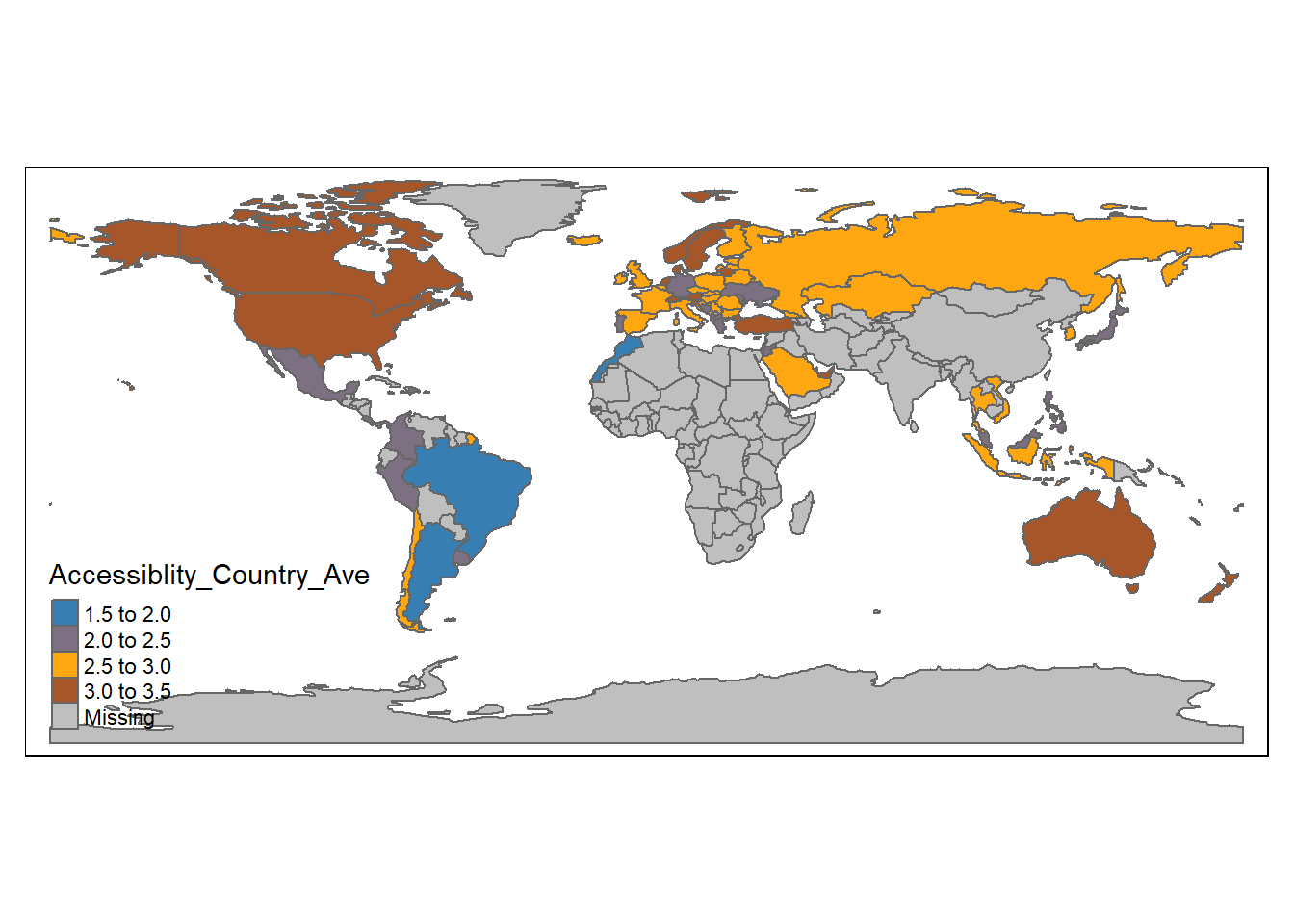

tm_shape(world_pisa) +
  tm_polygons(col="Human_Resource_ave",  palette = "Set1")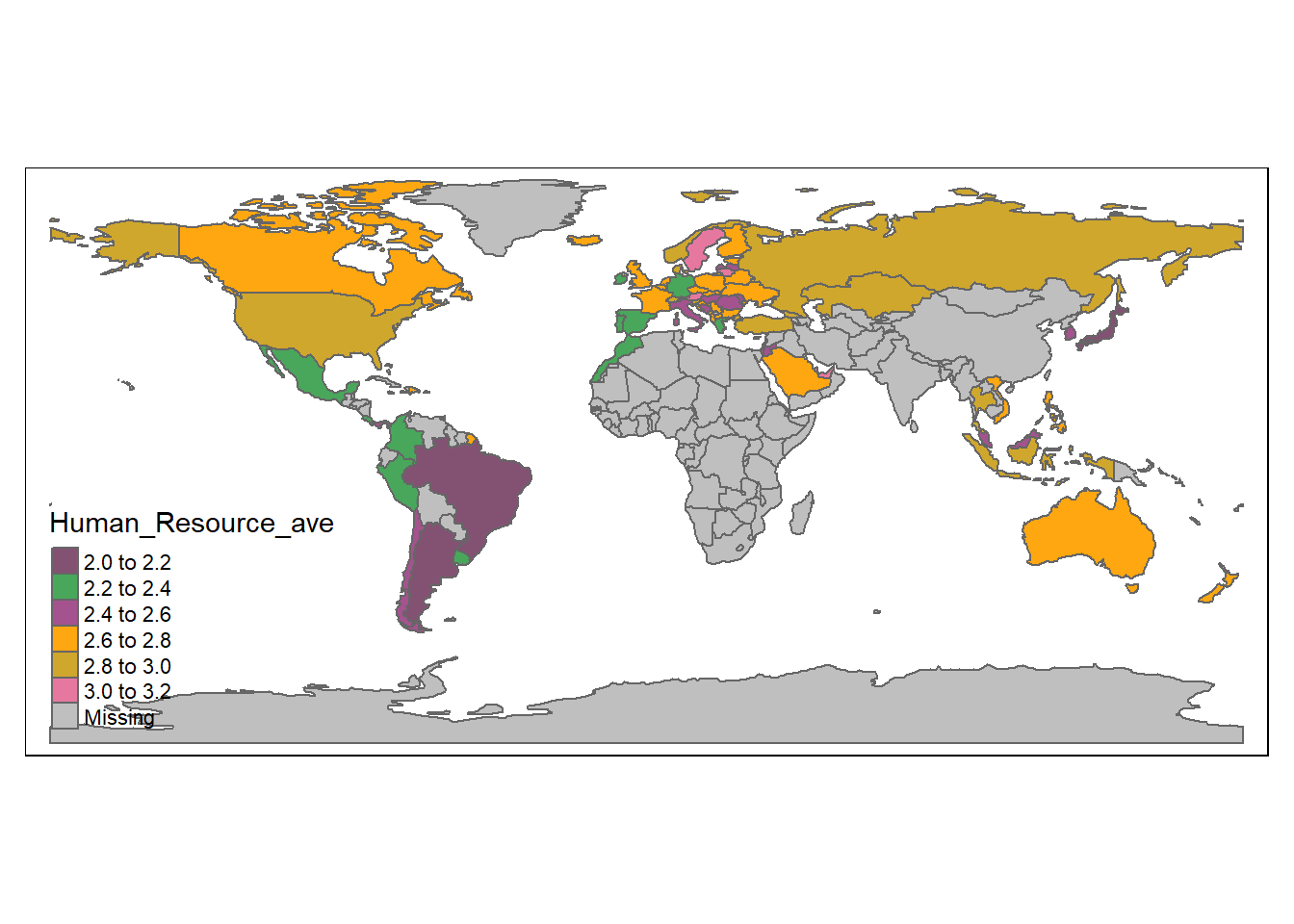

Finally, I create two world maps reflecting regional differences in terms of the accessibility to digital devices and the human resources support for them all over the world.Apparently, just a few countries have the grades higher than 3 points, which reflects that these countries’ agreement of enjoying good accessibility to digital devices.However, even some developed countries still expressed their limited accessibility to digital devices such as United Kingdom and France. The phenomenon, in fact, open the more questions and their answers will require further investigations on these country. I will take France and Unite Kingdom as case studies. With respect to “Human Resource Support,” most countries have reported the grades under 3 points. This may not disclose that these countries share the similar scenarios but there is no any objective measurements for them to measure their access to and human resources support on digital devices. Therefore, instead of reflecting that OECD countries lack human resources support, the data may show OECD and non-OECD countries have distinct expectations on human resources support. So self-report can only demonstrate the gap between their expectations and current situations.