duplicates of the latitute/longitudinal coordinates X, Y
SURVYEAR since we are only examining 2017-2018 survey
I thought I should delete: aggregate information that could be replicated: TOTFRL, TOTMENRTOTFENR, TOTAL, Member; HOWEVER, inspection of the median, range, and distribution of numeric variables in the summary indicates there are several mis-entries, (for example: student to teacher ratio: STUTERATIO has a min = 0, med = 15.3, and max=22350.
Some of the aggregate categories might help me check for mis-entries.
On the read in, I factored the ordinal variables:
GSHI, GSLO, SCHOOL_LEVEL, and ULOCALE
Code
#Work done to determine what to filter/recode on read in# PublicSchools_2017<-read_csv("_data/Public_School_Characteristics_2017-18.csv")%>%# select(-c("X", "Y","OBJECTID" ,"SURVYEAR"))#Aggregate variables I would have filtered if I wasn't concerned about mis-entries:#"TOTFRL", "TOTMENROL", "TOTFENROL", "MEMBER", "TOTAL"# Identify Levels for Factoring Ordinal Variables# #ULOCALE# PublicSchools_2017%>%# select(ULOCALE)%>%# unique()# #GSLO# PublicSchools_2017%>%# select(GSLO)%>%# unique()# #GSLHI# PublicSchools_2017%>%# select(GSHI)%>%# unique()# #SCHOOL_LEVEL# PublicSchools_2017%>%# select(SCHOOL_LEVEL)%>%# unique()#Recode all ordinal variable as factorsPublicSchools_2017<-read_csv("_data/Public_School_Characteristics_2017-18.csv")%>%select(-c("X", "Y","OBJECTID" ,"SURVYEAR")) %>%mutate(ULOCALE =recode_factor(ULOCALE,"11-City: Large"="City: Large","12-City: Mid-size"="City: Mid-size","13-City: Small"="City: Small","21-Suburb: Large"="Suburb: Large","22-Suburb: Mid-size"="Suburb: Mid-size","23-Suburb: Small"="Suburb: Small","31-Town: Fringe"="Town: Fringe","32-Town: Distant"="Town: Distant","33-Town: Remote"="Town: Remote","41-Rural: Fringe"="Rural: Fringe","42-Rural: Distant"="Rural: Distant","43-Rural: Remote"="Rural: Remote",.ordered =TRUE))%>%mutate(SCHOOL_LEVEL =recode_factor(SCHOOL_LEVEL,"Prekindergarten"="Prekindergarten","Elementary"="Elementary","Middle"="Middle","Secondary"="Secondary","High"="High","Ungraded"="Ungraded","Other"="Other","Not Applicable"="Not Applicable","Not Reported"="Not Reported",.ordered =TRUE))%>%mutate(GSLO =recode_factor(GSLO,"PK"="PK","KG"="KG","01"="01","02"="02","03"="03","04"="04","05"="05","M"="M","06"="06","07"="07","08"="08","09"="09","10"="10","11"="11","12"="12","AE"="AE","UG"="UG","N"="N",.ordered =TRUE))%>%mutate(GSHI =recode_factor(GSHI,"PK"="PK","KG"="KG","01"="01","02"="02","03"="03","04"="04","05"="05","M"="M","06"="06","07"="07","08"="08","09"="09","10"="10","11"="11","12"="12","13"="13","AE"="AE","UG"="UG","N"="N",.ordered =TRUE)) PublicSchools_2017
The PublicSchools_2017 data frame consists of data from selected questions from the 2017-208 National Teachers and Principals Survey conducted by the United States Census Board and is “a system of related questionnaires that provide descriptive data on the context of public and private elementary and secondary education in addition to giving local, state, and national policymakers a variety of statistics on the condition of education in the United States.”
Our data frame consists of a subset of the items surveyed from 100729 schools across the United States. The 75 variables contain information from the following categories:
Geographic Location of the School
State, town, and address
Level of Urbanization (rural, town, city, etc.)
Characteristics of the School design:
Charter, Magnet, Traditional Public,
Virtual/non
Highest and Lowest Grade levels served and number of students per grade level.
Level of School: Elementary, Middle, Secondary, Adult Ed., etc.
Type of School: Alternative, Regular school, Special education school, or Vocational school
Status of the school when surveyed (new, change of leadership, operational, etc.)
Student to Teacher Ratio
If the school has Title 1 status
Demographic Characteristics of the student body:
Number of students of given ethnic backgrounds by gender (M/F only)
Socioeconomic Characteristics of the student body:
Number of students qualifying for free or reduced lunch.
Questions for Further Review
What are the following variables?
G13
AS
UG: Ungraded (School level)
AE: Adult Education (School level)
FTE
STATUS
Why did the original Member have 2944 distinct values while total had 2944?
Code
# examine the summary to decide how to best set up our data frameprint(summarytools::dfSummary(PublicSchools_2017,varnumbers =FALSE,plain.ascii =FALSE,style ="grid",graph.magnif =0.70,valid.col =FALSE),method ='render',table.classes ='table-condensed')
Data Frame Summary
PublicSchools_2017
Dimensions: 100729 x 75
Duplicates: 0
Variable
Stats / Values
Freqs (% of Valid)
Graph
Missing
NCESSCH
[character]
1. 010000500870
2. 010000500871
3. 010000500879
4. 010000500889
5. 010000501616
6. 010000502150
7. 010000600193
8. 010000600872
9. 010000600876
10. 010000600877
[ 100719 others ]
1
(
0.0%
)
1
(
0.0%
)
1
(
0.0%
)
1
(
0.0%
)
1
(
0.0%
)
1
(
0.0%
)
1
(
0.0%
)
1
(
0.0%
)
1
(
0.0%
)
1
(
0.0%
)
100719
(
100.0%
)
0
(0.0%)
NMCNTY
[character]
1. Los Angeles County
2. Cook County
3. Maricopa County
4. Harris County
5. Orange County
6. Jefferson County
7. Montgomery County
8. Washington County
9. Wayne County
10. Dallas County
[ 1949 others ]
2264
(
2.2%
)
1388
(
1.4%
)
1256
(
1.2%
)
1142
(
1.1%
)
1074
(
1.1%
)
980
(
1.0%
)
888
(
0.9%
)
848
(
0.8%
)
817
(
0.8%
)
814
(
0.8%
)
89258
(
88.6%
)
0
(0.0%)
STABR
[character]
1. CA
2. TX
3. NY
4. FL
5. IL
6. MI
7. OH
8. PA
9. NC
10. NJ
[ 46 others ]
10323
(
10.2%
)
9320
(
9.3%
)
4808
(
4.8%
)
4375
(
4.3%
)
4245
(
4.2%
)
3734
(
3.7%
)
3610
(
3.6%
)
2990
(
3.0%
)
2691
(
2.7%
)
2595
(
2.6%
)
52038
(
51.7%
)
0
(0.0%)
LEAID
[character]
1. 7200030
2. 0622710
3. 1709930
4. 1200390
5. 3200060
6. 1200180
7. 1200870
8. 1500030
9. 4823640
10. 1201500
[ 17451 others ]
1121
(
1.1%
)
1009
(
1.0%
)
655
(
0.7%
)
537
(
0.5%
)
381
(
0.4%
)
336
(
0.3%
)
320
(
0.3%
)
294
(
0.3%
)
284
(
0.3%
)
268
(
0.3%
)
95524
(
94.8%
)
0
(0.0%)
ST_LEAID
[character]
1. PR-01
2. CA-1964733
3. IL-15-016-2990-25
4. FL-13
5. NV-02
6. FL-06
7. FL-29
8. HI-001
9. TX-101912
10. FL-50
[ 17451 others ]
1121
(
1.1%
)
1009
(
1.0%
)
655
(
0.7%
)
537
(
0.5%
)
381
(
0.4%
)
336
(
0.3%
)
320
(
0.3%
)
294
(
0.3%
)
284
(
0.3%
)
268
(
0.3%
)
95524
(
94.8%
)
0
(0.0%)
LEA_NAME
[character]
1. PUERTO RICO DEPARTMENT OF
2. Los Angeles Unified
3. City of Chicago SD 299
4. DADE
5. CLARK COUNTY SCHOOL DISTR
6. BROWARD
7. HILLSBOROUGH
8. Hawaii Department of Educ
9. HOUSTON ISD
10. PALM BEACH
[ 17147 others ]
1121
(
1.1%
)
1009
(
1.0%
)
655
(
0.7%
)
537
(
0.5%
)
381
(
0.4%
)
336
(
0.3%
)
320
(
0.3%
)
294
(
0.3%
)
284
(
0.3%
)
268
(
0.3%
)
95524
(
94.8%
)
0
(0.0%)
SCH_NAME
[character]
1. Lincoln Elementary School
2. Lincoln Elementary
3. Jefferson Elementary
4. Washington Elementary
5. Washington Elementary Sch
6. Central Elementary School
7. Jefferson Elementary Scho
8. Lincoln Elem School
9. Central High School
10. Roosevelt Elementary
[ 88366 others ]
64
(
0.1%
)
61
(
0.1%
)
53
(
0.1%
)
49
(
0.0%
)
46
(
0.0%
)
42
(
0.0%
)
33
(
0.0%
)
33
(
0.0%
)
32
(
0.0%
)
32
(
0.0%
)
100284
(
99.6%
)
0
(0.0%)
LSTREET1
[character]
1. 6420 E. Broadway Blvd. Su
2. Box DOE
3. 2405 FAIRVIEW SCHOOL RD
4. 1820 XENIUM LN N
5. Main St
6. 335 ALTERNATIVE LN
7. 2101 N TWYMAN RD
8. 720 9TH AVE
9. 50 Moreland Rd.
10. 951 W Snowflake Blvd
[ 92384 others ]
33
(
0.0%
)
28
(
0.0%
)
22
(
0.0%
)
19
(
0.0%
)
13
(
0.0%
)
12
(
0.0%
)
11
(
0.0%
)
11
(
0.0%
)
10
(
0.0%
)
10
(
0.0%
)
100560
(
99.8%
)
0
(0.0%)
LSTREET2
[character]
1. Suite B
2. Ste. 100
3. P.O. Box 1497
4. Suite A
5. Suite 200
6. Building B
7. Ste. 102
8. Ste. A
9. Suite 1
10. SUITE 111 HART
[ 482 others ]
8
(
1.4%
)
7
(
1.2%
)
6
(
1.0%
)
6
(
1.0%
)
5
(
0.8%
)
4
(
0.7%
)
4
(
0.7%
)
4
(
0.7%
)
4
(
0.7%
)
4
(
0.7%
)
540
(
91.2%
)
100137
(99.4%)
LSTREET3
[logical]
All NA's
100729
(100.0%)
LCITY
[character]
1. HOUSTON
2. Chicago
3. Los Angeles
4. BROOKLYN
5. SAN ANTONIO
6. Phoenix
7. BRONX
8. DALLAS
9. NEW YORK
10. Tucson
[ 14624 others ]
783
(
0.8%
)
664
(
0.7%
)
577
(
0.6%
)
569
(
0.6%
)
520
(
0.5%
)
446
(
0.4%
)
441
(
0.4%
)
378
(
0.4%
)
359
(
0.4%
)
330
(
0.3%
)
95662
(
95.0%
)
0
(0.0%)
LSTATE
[character]
1. CA
2. TX
3. NY
4. FL
5. IL
6. MI
7. OH
8. PA
9. NC
10. NJ
[ 45 others ]
10325
(
10.3%
)
9320
(
9.3%
)
4808
(
4.8%
)
4377
(
4.3%
)
4245
(
4.2%
)
3736
(
3.7%
)
3610
(
3.6%
)
2990
(
3.0%
)
2693
(
2.7%
)
2595
(
2.6%
)
52030
(
51.7%
)
0
(0.0%)
LZIP
[character]
1. 85710
2. 10456
3. 85364
4. 78521
5. 78572
6. 78577
7. 00731
8. 10457
9. 78539
10. 60623
[ 22526 others ]
53
(
0.1%
)
45
(
0.0%
)
44
(
0.0%
)
43
(
0.0%
)
42
(
0.0%
)
41
(
0.0%
)
39
(
0.0%
)
37
(
0.0%
)
37
(
0.0%
)
36
(
0.0%
)
100312
(
99.6%
)
0
(0.0%)
LZIP4
[character]
1. 8888
2. 1199
3. 1299
4. 9801
5. 2099
6. 1399
7. 1699
8. 1599
9. 1499
10. 1899
[ 8615 others ]
899
(
1.5%
)
113
(
0.2%
)
111
(
0.2%
)
106
(
0.2%
)
104
(
0.2%
)
101
(
0.2%
)
100
(
0.2%
)
99
(
0.2%
)
94
(
0.2%
)
89
(
0.2%
)
57411
(
96.9%
)
41502
(41.2%)
PHONE
[character]
1. (505)880-3744
2. (520)225-6060
3. (505)721-1051
4. (480)461-4000
5. (972)316-3663
6. (505)527-5800
7. (520)745-4588
8. (480)497-3300
9. (623)445-5000
10. (480)484-6100
[ 91818 others ]
141
(
0.1%
)
63
(
0.1%
)
36
(
0.0%
)
35
(
0.0%
)
34
(
0.0%
)
33
(
0.0%
)
33
(
0.0%
)
29
(
0.0%
)
28
(
0.0%
)
27
(
0.0%
)
100270
(
99.5%
)
0
(0.0%)
GSLO
[ordered, factor]
1. PK
2. KG
3. 01
4. 02
5. 03
6. 04
7. 05
8. M
9. 06
10. 07
[ 8 others ]
31179
(
31.0%
)
23839
(
23.7%
)
964
(
1.0%
)
606
(
0.6%
)
1581
(
1.6%
)
1165
(
1.2%
)
2578
(
2.6%
)
1113
(
1.1%
)
12912
(
12.8%
)
5441
(
5.4%
)
19351
(
19.2%
)
0
(0.0%)
GSHI
[ordered, factor]
1. PK
2. KG
3. 01
4. 02
5. 03
6. 04
7. 05
8. M
9. 06
10. 07
[ 9 others ]
1430
(
1.4%
)
526
(
0.5%
)
538
(
0.5%
)
1591
(
1.6%
)
1446
(
1.4%
)
3938
(
3.9%
)
28039
(
27.8%
)
1113
(
1.1%
)
10873
(
10.8%
)
499
(
0.5%
)
50736
(
50.4%
)
0
(0.0%)
VIRTUAL
[character]
1. A virtual school
2. Missing
3. Not a virtual school
4. Not Applicable
656
(
0.7%
)
183
(
0.2%
)
99049
(
98.3%
)
841
(
0.8%
)
0
(0.0%)
TOTFRL
[numeric]
Mean (sd) : 249.4 (275.2)
min ≤ med ≤ max:
-9 ≤ 178 ≤ 9626
IQR (CV) : 297 (1.1)
1906 distinct values
0
(0.0%)
FRELCH
[numeric]
Mean (sd) : 221.6 (253.9)
min ≤ med ≤ max:
-9 ≤ 149 ≤ 7581
IQR (CV) : 272 (1.1)
1765 distinct values
0
(0.0%)
REDLCH
[numeric]
Mean (sd) : 26 (36.9)
min ≤ med ≤ max:
-9 ≤ 16 ≤ 2045
IQR (CV) : 37 (1.4)
399 distinct values
0
(0.0%)
PK
[numeric]
Mean (sd) : 34.8 (53.5)
min ≤ med ≤ max:
0 ≤ 22 ≤ 1912
IQR (CV) : 43 (1.5)
468 distinct values
64621
(64.2%)
KG
[numeric]
Mean (sd) : 65 (46.9)
min ≤ med ≤ max:
0 ≤ 62 ≤ 948
IQR (CV) : 57 (0.7)
393 distinct values
43684
(43.4%)
G01
[numeric]
Mean (sd) : 64.4 (44.8)
min ≤ med ≤ max:
0 ≤ 62 ≤ 1408
IQR (CV) : 56 (0.7)
353 distinct values
43333
(43.0%)
G02
[numeric]
Mean (sd) : 64.6 (44.4)
min ≤ med ≤ max:
0 ≤ 63 ≤ 688
IQR (CV) : 56 (0.7)
345 distinct values
43268
(43.0%)
G03
[numeric]
Mean (sd) : 66.4 (46.3)
min ≤ med ≤ max:
0 ≤ 64 ≤ 783
IQR (CV) : 59 (0.7)
358 distinct values
43253
(42.9%)
G04
[numeric]
Mean (sd) : 67.9 (48.7)
min ≤ med ≤ max:
0 ≤ 65 ≤ 877
IQR (CV) : 61 (0.7)
382 distinct values
43470
(43.2%)
G05
[numeric]
Mean (sd) : 69.7 (56.7)
min ≤ med ≤ max:
0 ≤ 64 ≤ 985
IQR (CV) : 65 (0.8)
494 distinct values
44673
(44.3%)
G06
[numeric]
Mean (sd) : 91.5 (108.4)
min ≤ med ≤ max:
0 ≤ 56 ≤ 1155
IQR (CV) : 111 (1.2)
641 distinct values
58585
(58.2%)
G07
[numeric]
Mean (sd) : 102.7 (126.2)
min ≤ med ≤ max:
0 ≤ 52 ≤ 1439
IQR (CV) : 153 (1.2)
687 distinct values
63682
(63.2%)
G08
[numeric]
Mean (sd) : 101.9 (127.1)
min ≤ med ≤ max:
0 ≤ 50 ≤ 1608
IQR (CV) : 152 (1.2)
700 distinct values
63449
(63.0%)
G09
[numeric]
Mean (sd) : 124.7 (185.8)
min ≤ med ≤ max:
0 ≤ 40 ≤ 2799
IQR (CV) : 166 (1.5)
987 distinct values
68499
(68.0%)
G10
[numeric]
Mean (sd) : 120.4 (178.1)
min ≤ med ≤ max:
0 ≤ 39 ≤ 1837
IQR (CV) : 157 (1.5)
945 distinct values
68706
(68.2%)
G11
[numeric]
Mean (sd) : 115.4 (170.1)
min ≤ med ≤ max:
0 ≤ 40 ≤ 1719
IQR (CV) : 149 (1.5)
914 distinct values
68720
(68.2%)
G12
[numeric]
Mean (sd) : 114.1 (165.5)
min ≤ med ≤ max:
0 ≤ 43 ≤ 2580
IQR (CV) : 150 (1.5)
891 distinct values
68814
(68.3%)
G13
[logical]
1. FALSE
2. TRUE
36
(
97.3%
)
1
(
2.7%
)
100692
(100.0%)
TOTAL
[numeric]
Mean (sd) : 515.7 (450.2)
min ≤ med ≤ max:
0 ≤ 434 ≤ 14286
IQR (CV) : 408 (0.9)
2945 distinct values
2229
(2.2%)
MEMBER
[numeric]
Mean (sd) : 515.6 (449.9)
min ≤ med ≤ max:
0 ≤ 434 ≤ 14286
IQR (CV) : 408 (0.9)
2944 distinct values
2229
(2.2%)
AM
[numeric]
Mean (sd) : 6.7 (30.3)
min ≤ med ≤ max:
0 ≤ 1 ≤ 1395
IQR (CV) : 4 (4.5)
424 distinct values
20609
(20.5%)
HI
[numeric]
Mean (sd) : 142.5 (240.6)
min ≤ med ≤ max:
0 ≤ 49 ≤ 4677
IQR (CV) : 160 (1.7)
1745 distinct values
3852
(3.8%)
BL
[numeric]
Mean (sd) : 83 (151.4)
min ≤ med ≤ max:
0 ≤ 19 ≤ 5088
IQR (CV) : 90 (1.8)
1166 distinct values
8325
(8.3%)
WH
[numeric]
Mean (sd) : 247.9 (275.1)
min ≤ med ≤ max:
0 ≤ 182 ≤ 8146
IQR (CV) : 312 (1.1)
1839 distinct values
3993
(4.0%)
HP
[numeric]
Mean (sd) : 3.1 (24.7)
min ≤ med ≤ max:
0 ≤ 0 ≤ 1394
IQR (CV) : 2 (8)
305 distinct values
30008
(29.8%)
TR
[numeric]
Mean (sd) : 20.7 (27.3)
min ≤ med ≤ max:
0 ≤ 12 ≤ 1228
IQR (CV) : 24 (1.3)
307 distinct values
7137
(7.1%)
FTE
[numeric]
Mean (sd) : 32.6 (25.6)
min ≤ med ≤ max:
0 ≤ 27.6 ≤ 1419
IQR (CV) : 24 (0.8)
10066 distinct values
5233
(5.2%)
LATCOD
[numeric]
Mean (sd) : 37.8 (5.8)
min ≤ med ≤ max:
-14.3 ≤ 38.8 ≤ 71.3
IQR (CV) : 7.7 (0.2)
96746 distinct values
0
(0.0%)
LONCOD
[numeric]
Mean (sd) : -92.9 (16.9)
min ≤ med ≤ max:
-176.6 ≤ -89.3 ≤ 144.9
IQR (CV) : 20.2 (-0.2)
96911 distinct values
0
(0.0%)
ULOCALE
[ordered, factor]
1. City: Large
2. City: Mid-size
3. City: Small
4. Suburb: Large
5. Suburb: Mid-size
6. Suburb: Small
7. Town: Fringe
8. Town: Distant
9. Town: Remote
10. Rural: Fringe
[ 2 others ]
14851
(
14.7%
)
5876
(
5.8%
)
6635
(
6.6%
)
26772
(
26.6%
)
3305
(
3.3%
)
2053
(
2.0%
)
2963
(
2.9%
)
6266
(
6.2%
)
4138
(
4.1%
)
11179
(
11.1%
)
16691
(
16.6%
)
0
(0.0%)
STUTERATIO
[numeric]
Mean (sd) : 16.9 (85.7)
min ≤ med ≤ max:
0 ≤ 15.3 ≤ 22350
IQR (CV) : 5.3 (5.1)
3854 distinct values
6835
(6.8%)
STITLEI
[character]
1. Missing
2. No
3. Not Applicable
4. Yes
864
(
0.9%
)
14596
(
14.5%
)
29199
(
29.0%
)
56070
(
55.7%
)
0
(0.0%)
AMALM
[numeric]
Mean (sd) : 3.7 (16.1)
min ≤ med ≤ max:
0 ≤ 1 ≤ 743
IQR (CV) : 2 (4.4)
268 distinct values
26365
(26.2%)
AMALF
[numeric]
Mean (sd) : 3.6 (15.5)
min ≤ med ≤ max:
0 ≤ 1 ≤ 652
IQR (CV) : 2 (4.4)
263 distinct values
26708
(26.5%)
ASALM
[numeric]
Mean (sd) : 15.9 (45.2)
min ≤ med ≤ max:
0 ≤ 3 ≤ 1997
IQR (CV) : 11 (2.8)
522 distinct values
16162
(16.0%)
ASALF
[numeric]
Mean (sd) : 15.1 (42.5)
min ≤ med ≤ max:
0 ≤ 3 ≤ 1532
IQR (CV) : 11 (2.8)
495 distinct values
16080
(16.0%)
HIALM
[numeric]
Mean (sd) : 73.7 (123.5)
min ≤ med ≤ max:
0 ≤ 25 ≤ 2292
IQR (CV) : 83 (1.7)
1073 distinct values
4774
(4.7%)
HIALF
[numeric]
Mean (sd) : 70.5 (118.7)
min ≤ med ≤ max:
0 ≤ 24 ≤ 2461
IQR (CV) : 79 (1.7)
1047 distinct values
5121
(5.1%)
BLALM
[numeric]
Mean (sd) : 43.5 (77.3)
min ≤ med ≤ max:
0 ≤ 11 ≤ 2473
IQR (CV) : 48 (1.8)
687 distinct values
10801
(10.7%)
BLALF
[numeric]
Mean (sd) : 42.1 (76.8)
min ≤ med ≤ max:
0 ≤ 10 ≤ 2615
IQR (CV) : 46 (1.8)
693 distinct values
11485
(11.4%)
WHALM
[numeric]
Mean (sd) : 128.6 (140.5)
min ≤ med ≤ max:
0 ≤ 95 ≤ 3854
IQR (CV) : 160 (1.1)
1046 distinct values
4502
(4.5%)
WHALF
[numeric]
Mean (sd) : 120.8 (135.6)
min ≤ med ≤ max:
0 ≤ 88 ≤ 4292
IQR (CV) : 152 (1.1)
1030 distinct values
4682
(4.6%)
HPALM
[numeric]
Mean (sd) : 1.7 (13.4)
min ≤ med ≤ max:
0 ≤ 0 ≤ 751
IQR (CV) : 1 (7.9)
210 distinct values
34182
(33.9%)
HPALF
[numeric]
Mean (sd) : 1.6 (12.2)
min ≤ med ≤ max:
0 ≤ 0 ≤ 643
IQR (CV) : 1 (7.7)
212 distinct values
34563
(34.3%)
TRALM
[numeric]
Mean (sd) : 10.8 (13.9)
min ≤ med ≤ max:
0 ≤ 6 ≤ 512
IQR (CV) : 13 (1.3)
174 distinct values
9200
(9.1%)
TRALF
[numeric]
Mean (sd) : 10.5 (14)
min ≤ med ≤ max:
0 ≤ 6 ≤ 716
IQR (CV) : 12 (1.3)
183 distinct values
9477
(9.4%)
TOTMENROL
[numeric]
Mean (sd) : 264.9 (229)
min ≤ med ≤ max:
0 ≤ 224 ≤ 6890
IQR (CV) : 210 (0.9)
1691 distinct values
2296
(2.3%)
TOTFENROL
[numeric]
Mean (sd) : 251.1 (222.8)
min ≤ med ≤ max:
0 ≤ 211 ≤ 7396
IQR (CV) : 200 (0.9)
1646 distinct values
2362
(2.3%)
STATUS
[numeric]
Mean (sd) : 1.1 (0.6)
min ≤ med ≤ max:
1 ≤ 1 ≤ 8
IQR (CV) : 0 (0.5)
1
:
98557
(
97.8%
)
3
:
1103
(
1.1%
)
4
:
77
(
0.1%
)
5
:
110
(
0.1%
)
6
:
500
(
0.5%
)
7
:
341
(
0.3%
)
8
:
41
(
0.0%
)
0
(0.0%)
UG
[numeric]
Mean (sd) : 11.2 (33.6)
min ≤ med ≤ max:
0 ≤ 2 ≤ 1017
IQR (CV) : 10 (3)
217 distinct values
88689
(88.0%)
AE
[logical]
1. FALSE
2. TRUE
60
(
93.8%
)
4
(
6.2%
)
100665
(99.9%)
SCHOOL_TYPE_TEXT
[character]
1. Alternative/other school
2. Regular school
3. Special education school
4. Vocational school
5531
(
5.5%
)
91737
(
91.1%
)
1948
(
1.9%
)
1513
(
1.5%
)
0
(0.0%)
SY_STATUS_TEXT
[character]
1. Currently operational
2. New school
3. School has changed agency
4. School has reopened
5. School temporarily closed
6. School to be operational
7. School was operational bu
98557
(
97.8%
)
1103
(
1.1%
)
110
(
0.1%
)
41
(
0.0%
)
500
(
0.5%
)
341
(
0.3%
)
77
(
0.1%
)
0
(0.0%)
SCHOOL_LEVEL
[ordered, factor]
1. Prekindergarten
2. Elementary
3. Middle
4. Secondary
5. High
6. Ungraded
7. Other
8. Not Applicable
9. Not Reported
10. Adult Education
1430
(
1.4%
)
53287
(
52.9%
)
16506
(
16.4%
)
602
(
0.6%
)
22977
(
22.8%
)
166
(
0.2%
)
3824
(
3.8%
)
796
(
0.8%
)
1113
(
1.1%
)
28
(
0.0%
)
0
(0.0%)
AS
[numeric]
Mean (sd) : 29.8 (85.8)
min ≤ med ≤ max:
0 ≤ 5 ≤ 3529
IQR (CV) : 21 (2.9)
850 distinct values
12717
(12.6%)
CHARTER_TEXT
[character]
1. No
2. Not Applicable
3. Yes
87007
(
86.4%
)
6387
(
6.3%
)
7335
(
7.3%
)
0
(0.0%)
MAGNET_TEXT
[character]
1. Missing
2. No
3. Not Applicable
4. Yes
6256
(
6.2%
)
77531
(
77.0%
)
13520
(
13.4%
)
3422
(
3.4%
)
0
(0.0%)
Generated by summarytools 1.0.1 (R version 4.2.1) 2022-12-21
Because we have survey data, we will have a relatively wide data frame, and will have to make use of select and group by when making summaries or visualizations.
The ULOCALE variable needed to be recoded as an ordinal variable with levels in order to have the bars appear in the appropriate order for our visualization.
Upon closer inspection, it turns out that there are several numeric variables with data mis-entered:
The number of students with Free or Reduced lunch cannot be negative
Student to Teacher Ratio cannot exceed 100 (yet there entries in 600 and even 2350)
How should these values be recoded, so we can still use the information for a given school but not throw off our summary statistics or visual representations?
The min, median, max values are suspicious for several of the numeric entries. If I had more time, I would consider each variable, what I know about it in context, and take advantage of mean/sd or median and IQR to replace likely mis-entries with N/A
I used the code below to remove the most extreme cases from our calculations based on the logical bounds of a ratio and count of students as well as knowledge of classroom sizes in the US.
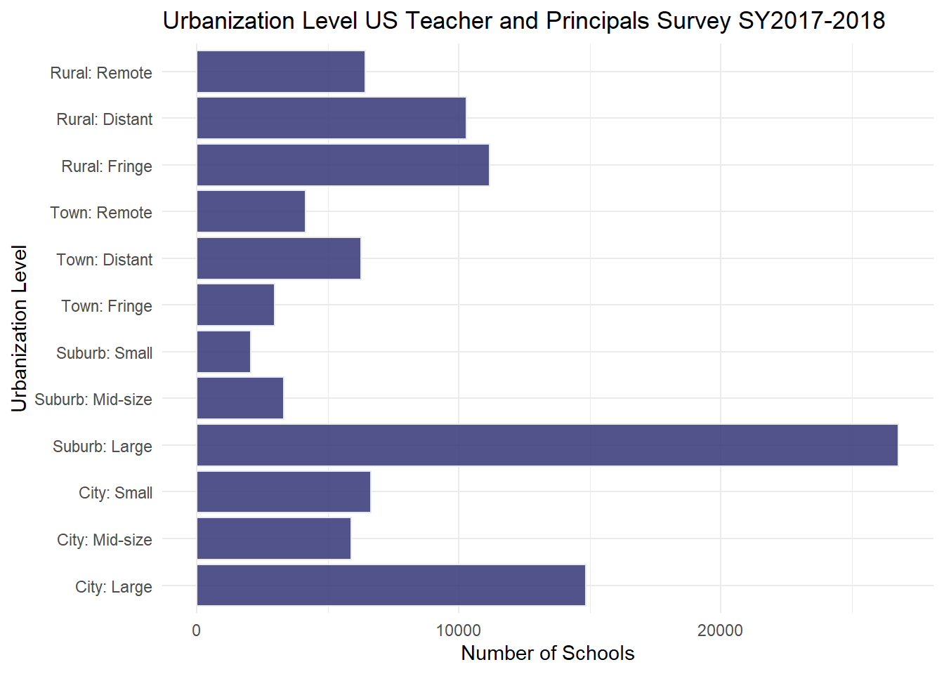
I chose to visualize the ULOCALE using a geom_bar since it was an ordinal variable. Before, creating the bar chart, I factored and ordered the values for each of the urbanization classifications from the survey. Because the variable names were rather long, I “flipped” the orientation of the chart to horizontal in order to make the names easier to read.
It is striking to see how there are many more Large Suburban Schools in our country, relative to the other urbanization levels.
Code
# Bar Chart School Levelggplot(PublicSchools_2017, aes(ULOCALE)) +geom_bar(fill="#404080", color="#e8ecef", alpha=0.9) +#geom_bar(stat="identity", width=2) + scale_fill_manual("legend", values =c("City: Large"="blue", "City: Mid-Size"="blue", "City: Small"="blue")) +theme_minimal() +labs(title ="Urbanization Level US Teacher and Principals Survey SY2017-2018", y ="Number of Schools", x ="Urbanization Level") +coord_flip()
Code
# Perhaps histogram of urban status
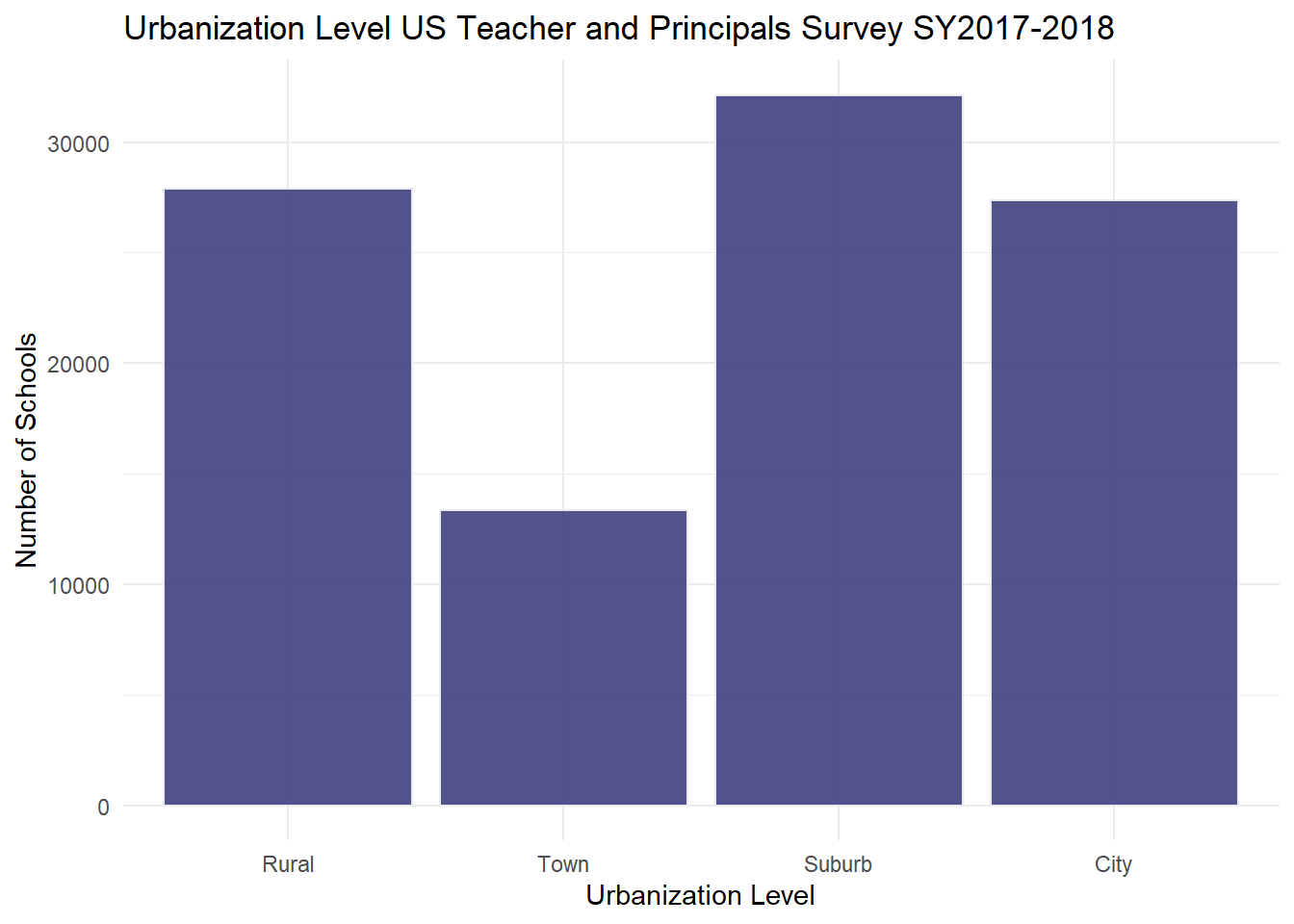
Are most schools classified as suburban? To answer this question, I collapsed the Rural, City, Town, and Suburban categories and created a second chart. While, there are still the most suburban schools represented, one can see that the majority of US public schools are either located in Suburban, City, or Rural regions.
# Bar Broader Urbanization Levelggplot(Urbanization, aes(UrbBroad)) +geom_bar(fill="#404080", color="#e8ecef", alpha=0.9) +#geom_bar(stat="identity", width=2) + theme_minimal() +labs(title ="Urbanization Level US Teacher and Principals Survey SY2017-2018", y ="Number of Schools", x ="Urbanization Level")
Code
#coord_flip()
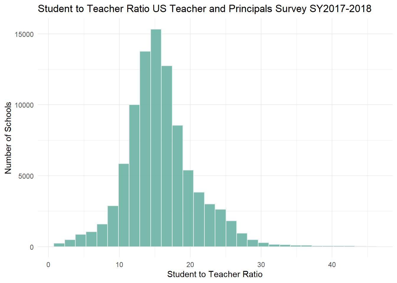
I decided to use a histogram to to visualize the distribution of the student to teacher ratio in schools across the country. From this we can have an idea of the distribution of class sizes across the United States. We see a symmetric distribution with most frequent ratio being between 15-16 students per teacher.
Code
ggplot(PublicSchools_2017, aes(x = STUTERATIO)) +geom_histogram(fill="#69b3a2", color="#e9ecef", alpha=0.9) +theme_minimal() +labs(title ="Student to Teacher Ratio US Teacher and Principals Survey SY2017-2018",y ="Number of Schools", x ="Student to Teacher Ratio")
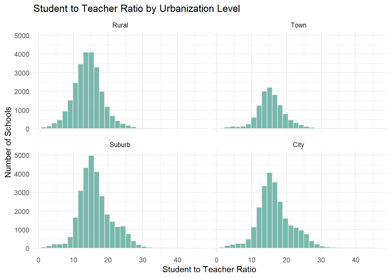
One might consider if the distribution of the student to teacher ratio is different based on the urbanization level of a school, i.e. “Are students in City Schools more likely to be in crowded classrooms?”. I would like to produce a more advanced plot, where I see 4 histograms side by side where I group this data by Rural/Town/Suburban/City Urban level.
Here we can see that all urban levels seem to have the most schools with a student to teacher between 14-16 BUT urban and suburban schools show a left skew, and have a higher proportion of schools with a student to teacher ratio greater than 16.
ggplot(Urban_Ratio, aes(x = STUTERATIO)) +geom_histogram( fill="#69b3a2", color="#e9ecef", alpha=0.9) +labs(title ="Student to Teacher Ratio by Urbanization Level", y ="Number of Schools",x ="Student to Teacher Ratio") +theme_minimal() +facet_wrap(vars(UrbBroad))
Questions
How do I change the colors of individual bars in my first chart so that all of the “City Bars” were one color, “Suburban Bars” another, and “Rural Bars” another.
When I originally tried to create this histogram, I noticed that the bin-sizes were off. It turns out that there are some mis-entries in the STUTERATIO column. Notably: a school with a STUTERATIO of 677.36 and another with a ratio of 22350. These are clearly mis-entries. What would be the best way to re-code these? I used some knowledge of percents and classroom size to filter the values.
If I don’t have background knowledge, should I use the Median/IQR, or iteratively use the Mean/3SD to remove outliers?
(leaving this link here for future reference) R Graph Gallery
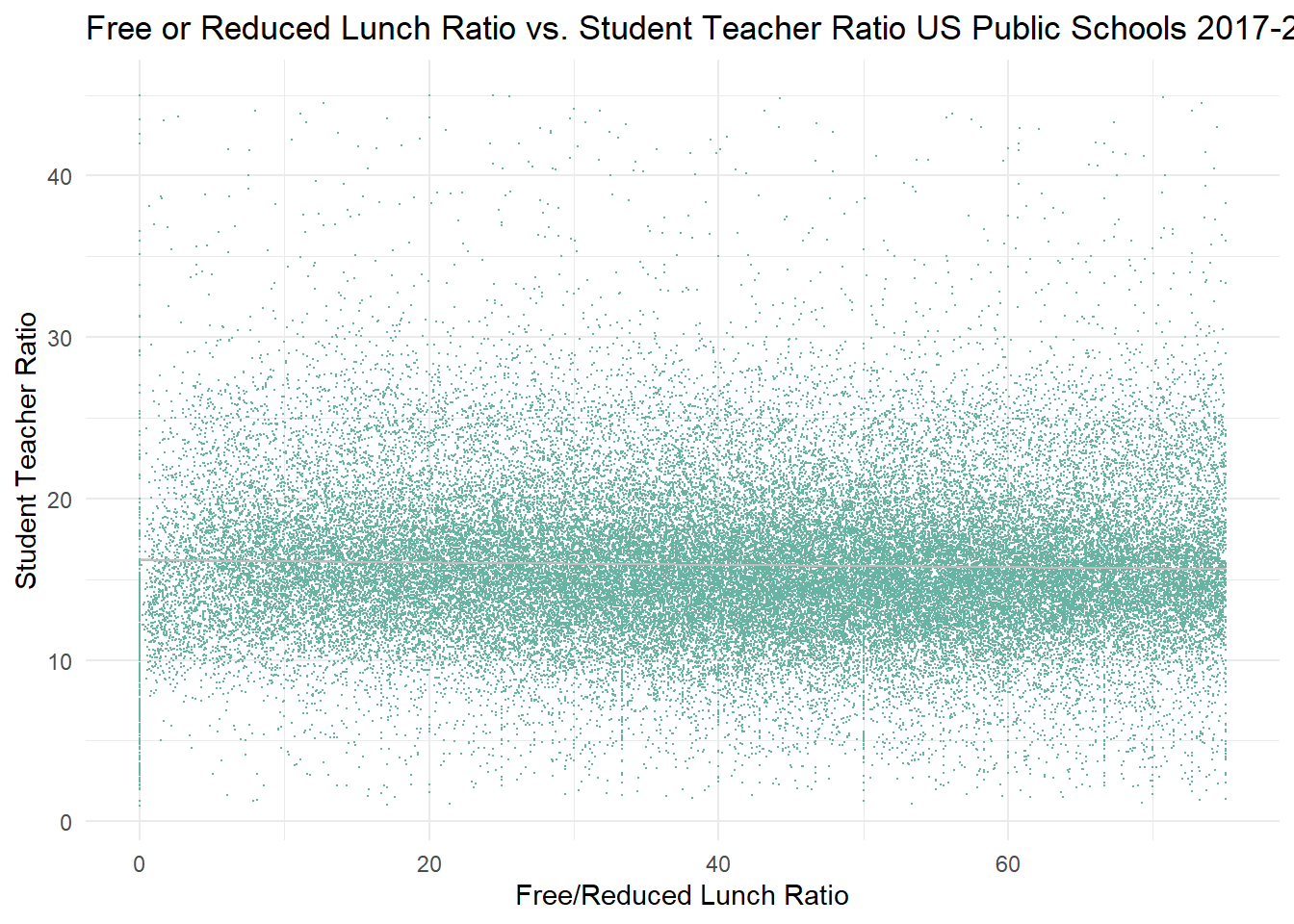
I chose to visualize the percentage of students qualifying for either free or reduced lunch at a school against the student to teacher ratio. I was curious to see if there appears to be an association between socio-economic status of the student body of a schoo and the student to teacher ratio. When examining the values of FRELCH and REDLCH in the summary, I realized there were several apparent mis-entries. Before producing the scatter plot, I first attempted to filter out data mis-entries.
Code
# Comparing Student Teacher Ratio to Free Reduced Lunch Ratio and removing FRED_Lunch_Teach <-PublicSchools_2017%>%select(FRELCH, STUTERATIO, REDLCH, TOTAL )%>%mutate(Ratio_FRED_LCH = (FRELCH + REDLCH)/TOTAL*100)%>%mutate(Ratio_FRED_LCH =replace(Ratio_FRED_LCH, which(Ratio_FRED_LCH>75), NA))%>%mutate(Ratio_FRED_LCH =replace(Ratio_FRED_LCH, which(Ratio_FRED_LCH<0), NA))FRED_Lunch_Teach
Code
ggplot(FRED_Lunch_Teach, aes(x=Ratio_FRED_LCH, y=STUTERATIO)) +geom_point(size = .05, color="#69b3a2")+geom_smooth(method="lm",color="grey", size =.5 )+labs(title ="Free or Reduced Lunch Ratio vs. Student Teacher Ratio US Public Schools 2017-2018", y ="Student Teacher Ratio",x ="Free/Reduced Lunch Ratio") +theme_minimal()
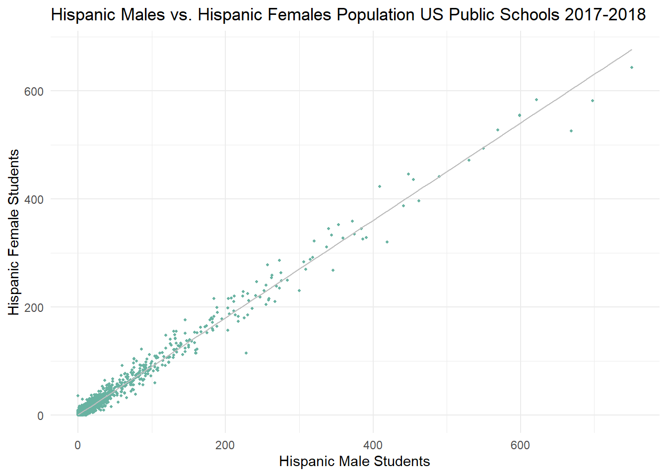
I also produced a scatter plot of Hispanic Male pop vs. Hispanic Female pop. in schools. This is not interesting from an analysis perspective; I performed this as a sanity check for myself to see if my graph showed a strong linear correlation.
Code
# Comparing Number of Hispanic Male Students to Hispanic Female Studentsggplot(PublicSchools_2017, aes(x=HPALM, y=HPALF)) +geom_point(size=.65, color="#69b3a2" )+geom_smooth(method="lm",color="grey", size =.5 )+labs(title ="Hispanic Males vs. Hispanic Females Population US Public Schools 2017-2018", y ="Hispanic Female Students",x ="Hispanic Male Students") +theme_minimal()
Since this data set had latitude and longitudinal data for the geographic locations of the schools, it would be great to practice making a map with the info.
---title: "Challenge 5"author: "Theresa Szczepanski"description: "Introduction to Visualization"date: "10/05/2022"format: html: toc: true code-copy: true code-tools: true df-print: paged code-fold: truecategories: - Theresa_Szczepanski - challenge_5 - public_schools---```{r}#| label: setup#| warning: false#| message: falselibrary(tidyverse)library(ggplot2)knitr::opts_chunk$set(echo =TRUE, warning=FALSE, message=FALSE)```::: panel-tabset## Public School Characteristics ⭐⭐⭐⭐ ::: panel-tabset### Read in the DataOn the read in, I deleted: - duplicates of the latitute/longitudinal coordinates `X`, `Y` - `SURVYEAR` since we are only examining 2017-2018 survey - __I thought I should delete__: aggregate information that could be replicated: `TOTFRL`, `TOTMENR``TOTFENR`, `TOTAL`, `Member`; __HOWEVER__, inspection of the median, range, and distribution of numeric variables in the summary indicates there are several mis-entries, (for example: student to teacher ratio: `STUTERATIO` has a min = 0, med = 15.3, and max=22350.- Some of the aggregate categories might help me check for mis-entries.On the read in, I factored the ordinal variables: - `GSHI`, `GSLO`, `SCHOOL_LEVEL`, and `ULOCALE````{r}#Work done to determine what to filter/recode on read in# PublicSchools_2017<-read_csv("_data/Public_School_Characteristics_2017-18.csv")%>%# select(-c("X", "Y","OBJECTID" ,"SURVYEAR"))#Aggregate variables I would have filtered if I wasn't concerned about mis-entries:#"TOTFRL", "TOTMENROL", "TOTFENROL", "MEMBER", "TOTAL"# Identify Levels for Factoring Ordinal Variables# #ULOCALE# PublicSchools_2017%>%# select(ULOCALE)%>%# unique()# #GSLO# PublicSchools_2017%>%# select(GSLO)%>%# unique()# #GSLHI# PublicSchools_2017%>%# select(GSHI)%>%# unique()# #SCHOOL_LEVEL# PublicSchools_2017%>%# select(SCHOOL_LEVEL)%>%# unique()#Recode all ordinal variable as factorsPublicSchools_2017<-read_csv("_data/Public_School_Characteristics_2017-18.csv")%>%select(-c("X", "Y","OBJECTID" ,"SURVYEAR")) %>%mutate(ULOCALE =recode_factor(ULOCALE,"11-City: Large"="City: Large","12-City: Mid-size"="City: Mid-size","13-City: Small"="City: Small","21-Suburb: Large"="Suburb: Large","22-Suburb: Mid-size"="Suburb: Mid-size","23-Suburb: Small"="Suburb: Small","31-Town: Fringe"="Town: Fringe","32-Town: Distant"="Town: Distant","33-Town: Remote"="Town: Remote","41-Rural: Fringe"="Rural: Fringe","42-Rural: Distant"="Rural: Distant","43-Rural: Remote"="Rural: Remote",.ordered =TRUE))%>%mutate(SCHOOL_LEVEL =recode_factor(SCHOOL_LEVEL,"Prekindergarten"="Prekindergarten","Elementary"="Elementary","Middle"="Middle","Secondary"="Secondary","High"="High","Ungraded"="Ungraded","Other"="Other","Not Applicable"="Not Applicable","Not Reported"="Not Reported",.ordered =TRUE))%>%mutate(GSLO =recode_factor(GSLO,"PK"="PK","KG"="KG","01"="01","02"="02","03"="03","04"="04","05"="05","M"="M","06"="06","07"="07","08"="08","09"="09","10"="10","11"="11","12"="12","AE"="AE","UG"="UG","N"="N",.ordered =TRUE))%>%mutate(GSHI =recode_factor(GSHI,"PK"="PK","KG"="KG","01"="01","02"="02","03"="03","04"="04","05"="05","M"="M","06"="06","07"="07","08"="08","09"="09","10"="10","11"="11","12"="12","13"="13","AE"="AE","UG"="UG","N"="N",.ordered =TRUE)) PublicSchools_2017```::: panel-tabset### Briefly describe the dataThe `PublicSchools_2017` data frame consists of data from selected questions from the [2017-208 National Teachers and Principals Survey](https://nces.ed.gov/surveys/ntps/question1718.asp)conducted by the United States Census Board and is "a system of related questionnaires that provide descriptive data on the context of public and private elementary and secondary education in addition to giving local, state, and national policymakers a variety of statistics on the condition of education in the United States."Our data frame consists of a subset of the items surveyed from 100729 schools across the United States. The 75 variables contain information from the following categories:Geographic Location of the School- State, town, and address- Level of Urbanization (rural, town, city, etc.)Characteristics of the School design:- Charter, Magnet, Traditional Public, - Virtual/non- Highest and Lowest Grade levels served and number of students per grade level.- Level of School: Elementary, Middle, Secondary, Adult Ed., etc.- Type of School: Alternative, Regular school, Special education school, or Vocational school - Status of the school when surveyed (new, change of leadership, operational, etc.)- Student to Teacher Ratio- If the school has Title 1 statusDemographic Characteristics of the student body:- Number of students of given ethnic backgrounds by gender (M/F only)Socioeconomic Characteristics of the student body:- Number of students qualifying for free or reduced lunch.## Questions for Further ReviewWhat are the following variables? - `G13` - `AS` - `UG`: Ungraded (School level) - `AE`: Adult Education (School level) - `FTE` - `STATUS`Why did the original `Member` have 2944 distinct values while `total` had 2944?### Data Summary```{r}# examine the summary to decide how to best set up our data frameprint(summarytools::dfSummary(PublicSchools_2017,varnumbers =FALSE,plain.ascii =FALSE,style ="grid",graph.magnif =0.70,valid.col =FALSE),method ='render',table.classes ='table-condensed')```:::### Tidy Data (MUCH WORK LEFT HERE)Because we have survey data, we will have a relatively wide data frame, and will have to make use of `select` and `group by` when making summaries or visualizations.The `ULOCALE` variable needed to be recoded as an ordinal variable with levels in order to have the bars appear in the appropriate order for our visualization.Upon closer inspection, it turns out that there are several numeric variables withdata mis-entered:- The number of students with Free or Reduced lunch cannot be negative- Student to Teacher Ratio cannot exceed 100 (yet there entries in 600 and even 2350)- How should these values be recoded, so we can still use the information for a given school but not throw off our summary statistics or visual representations?- The min, median, max values are suspicious for several of the numeric entries. If I had more time, I would consider each variable, what I know about it in context, and take advantage of mean/sd or median and IQR to replace likely mis-entries with N/A- I used the code below to remove the most extreme cases from our calculations based on the logical bounds of a ratio and count of students as well as knowledge of classroom sizes in the US.```{r}PublicSchools_2017<-PublicSchools_2017%>%mutate(FRELCH =replace(FRELCH, which(FRELCH<0), NA))%>%mutate(REDLCH =replace(REDLCH, which(REDLCH<0), NA))%>%mutate(STUTERATIO =replace(STUTERATIO, which(STUTERATIO>45), NA))%>%mutate(STUTERATIO =replace(STUTERATIO, which(STUTERATIO<1), NA))```### Univariate VisualizationsI chose to visualize the `ULOCALE` using a `geom_bar` since it was an ordinal variable. Before, creating the bar chart, I factored and ordered the values for each of the urbanization classifications from the survey. Because the variablenames were rather long, I "flipped" the orientation of the chart to horizontal in order to make the names easier to read.It is striking to see how there are many more __Large Suburban Schools__in our country, relative to the other urbanization levels.```{r}# Bar Chart School Levelggplot(PublicSchools_2017, aes(ULOCALE)) +geom_bar(fill="#404080", color="#e8ecef", alpha=0.9) +#geom_bar(stat="identity", width=2) + scale_fill_manual("legend", values =c("City: Large"="blue", "City: Mid-Size"="blue", "City: Small"="blue")) +theme_minimal() +labs(title ="Urbanization Level US Teacher and Principals Survey SY2017-2018", y ="Number of Schools", x ="Urbanization Level") +coord_flip()# Perhaps histogram of urban status```Are most schools classified as suburban? To answer this question, I collapsed the Rural, City, Town, and Suburban categories and created a second chart. While, thereare still the most suburban schools represented, one can see that the majority of US public schools are either located in Suburban, City, or Rural regions.```{r}Urbanization <-PublicSchools_2017%>%select(ULOCALE)%>%mutate(UrbBroad =ifelse(str_detect(ULOCALE,"Rural"), "Rural", ifelse(str_detect(ULOCALE, "Town"),"Town", ifelse(str_detect(ULOCALE, "Suburb"),"Suburb", ifelse(str_detect(ULOCALE, "City"),"City", ULOCALE)))))%>%mutate(UrbBroad =recode_factor(UrbBroad,"Rural"="Rural","Town"="Town","Suburb"="Suburb","City"="City",.ordered =TRUE)) Urbanization# Bar Broader Urbanization Levelggplot(Urbanization, aes(UrbBroad)) +geom_bar(fill="#404080", color="#e8ecef", alpha=0.9) +#geom_bar(stat="identity", width=2) + theme_minimal() +labs(title ="Urbanization Level US Teacher and Principals Survey SY2017-2018", y ="Number of Schools", x ="Urbanization Level") #coord_flip()```I decided to use a histogram to to visualize the distribution of the student to teacher ratio in schools across the country. From this we can have an idea of the distribution of class sizes across the United States. We see a symmetric distribution with most frequent ratio being between 15-16 students per teacher.```{r}ggplot(PublicSchools_2017, aes(x = STUTERATIO)) +geom_histogram(fill="#69b3a2", color="#e9ecef", alpha=0.9) +theme_minimal() +labs(title ="Student to Teacher Ratio US Teacher and Principals Survey SY2017-2018",y ="Number of Schools", x ="Student to Teacher Ratio")``` One might consider if the distribution of the student to teacher ratio is different based on the urbanization level of a school, i.e. "Are students in City Schools more likely to be in crowded classrooms?". I would like to produce a more advanced plot, where I see 4 histograms side by side where I group this data by Rural/Town/Suburban/City Urban level. Here we can see that all urban levels seem to have the most schools with a student to teacher between 14-16 BUT urban and suburban schools show a left skew, and have a higher proportion of schools with a student to teacher ratio greater than 16.```{r}Urban_Ratio <-PublicSchools_2017%>%select(ULOCALE, STUTERATIO)%>%mutate(UrbBroad =ifelse(str_detect(ULOCALE,"Rural"), "Rural", ifelse(str_detect(ULOCALE, "Town"),"Town", ifelse(str_detect(ULOCALE, "Suburb"),"Suburb", ifelse(str_detect(ULOCALE, "City"),"City", ULOCALE)))))%>%mutate(UrbBroad =recode_factor(UrbBroad,"Rural"="Rural","Town"="Town","Suburb"="Suburb","City"="City",.ordered =TRUE)) Urban_Ratioggplot(Urban_Ratio, aes(x = STUTERATIO)) +geom_histogram( fill="#69b3a2", color="#e9ecef", alpha=0.9) +labs(title ="Student to Teacher Ratio by Urbanization Level", y ="Number of Schools",x ="Student to Teacher Ratio") +theme_minimal() +facet_wrap(vars(UrbBroad))```## QuestionsHow do I change the colors of individual bars in my first chart so that all of the "City Bars" were one color, "Suburban Bars" another, and "Rural Bars" another.When I originally tried to create this histogram, I noticed that the bin-sizes were off. It turns out that there are some mis-entries in the `STUTERATIO` column. Notably: a school with a STUTERATIO of 677.36 and another with a ratio of 22350. These are clearly mis-entries. What would be the best way to re-code these? I used some knowledge of percents and classroom size to filter the values. If I don't have background knowledge, should I use the Median/IQR, or iteratively use the Mean/3SD to remove outliers?(leaving this link here for future reference)[R Graph Gallery](https://r-graph-gallery.com/)### Bivariate Visualization(s)I chose to visualize the percentage of students qualifying for either free or reduced lunch at a school against the student to teacher ratio. I was curious to see if there appears to be an association between socio-economic status of the student body of a schoo and the student to teacher ratio. When examining the valuesof `FRELCH` and `REDLCH` in the summary, I realized there were several apparent mis-entries. Before producing the scatter plot, I first attempted to filter out data mis-entries.```{r}# Comparing Student Teacher Ratio to Free Reduced Lunch Ratio and removing FRED_Lunch_Teach <-PublicSchools_2017%>%select(FRELCH, STUTERATIO, REDLCH, TOTAL )%>%mutate(Ratio_FRED_LCH = (FRELCH + REDLCH)/TOTAL*100)%>%mutate(Ratio_FRED_LCH =replace(Ratio_FRED_LCH, which(Ratio_FRED_LCH>75), NA))%>%mutate(Ratio_FRED_LCH =replace(Ratio_FRED_LCH, which(Ratio_FRED_LCH<0), NA))FRED_Lunch_Teachggplot(FRED_Lunch_Teach, aes(x=Ratio_FRED_LCH, y=STUTERATIO)) +geom_point(size = .05, color="#69b3a2")+geom_smooth(method="lm",color="grey", size =.5 )+labs(title ="Free or Reduced Lunch Ratio vs. Student Teacher Ratio US Public Schools 2017-2018", y ="Student Teacher Ratio",x ="Free/Reduced Lunch Ratio") +theme_minimal()```I also produced a scatter plot of Hispanic Male pop vs. Hispanic Female pop. in schools. This is not interesting from an analysis perspective; I performed this as a sanity check for myself to see if my graph showed a strong linear correlation.```{r}# Comparing Number of Hispanic Male Students to Hispanic Female Studentsggplot(PublicSchools_2017, aes(x=HPALM, y=HPALF)) +geom_point(size=.65, color="#69b3a2" )+geom_smooth(method="lm",color="grey", size =.5 )+labs(title ="Hispanic Males vs. Hispanic Females Population US Public Schools 2017-2018", y ="Hispanic Female Students",x ="Hispanic Male Students") +theme_minimal()``````{r}# testing cross tabs#xtabs(~ GSLO + GSHI, PublicSchools_2017)```### Fun Mapping VisualizationSince this data set had latitude and longitudinal data for the geographic locationsof the schools, it would be great to practice making a map with the info.```{r}#PublicSchools_2017MAP<- st_as_sf(PublicSchools_2017, coords = c("LONCOD", "LATCOD"), crs = 4326)```## QuestionsHow do I get the mapping visualization to work?::::::