SchoolID : There are several variables that identify our school, I removed all but one, testschoolcode.
StudentPrivacy: I left the sasid variable which is a student identifier number, but eliminated all values corresponding to students’ names.
dis: We are a charter school within our own unique district, therefore any “district level” data is identical to our “school level” data.
Rename
I currently have not renamed variables, but I have a list of variables for which I need to talk with my administration to access a key to understand what they represent. Ideally, after this, I would put
an E_ before all ELA MCAS student performance metric variables
an M_ before all Math MCAS student performance metric variables
an S_ before all Science MCAS student performance metric variables
an SI_ before all student demographic characteristic identifying variables
Mutate
I left as doubles
variables that measured scores on specific MCAS items e.g., mitem1
variables that measured student growth percentiles (sgp)
variables that counted a student’s years in the school system or state.
Recode to char
variables that are nominal, e.g., town
Refactor as ord
variables that are ordinal, e.g., mperflev.
Recode to date
-dob using lubridate.
Code
#Filter, rename variables, and mutate values of variables on read-inMCAS_2022<-read_csv("_data/PrivateSpring2022_MCAS_full_preliminary_results_04830305.csv",skip=1)%>%select(-c("sprp_dis", "sprp_sch", "sprp_dis_name", "sprp_sch_name", "sprp_orgtype","schtype", "testschoolname", "yrsindis", "conenr_dis"))%>%#Recode all nominal variables as charactersmutate(testschoolcode =as.character(testschoolcode))%>%# mutate(sasid = as.character(sasid))%>%mutate(highneeds =as.character(highneeds))%>%mutate(lowincome =as.character(lowincome))%>%mutate(title1 =as.character(title1))%>%mutate(ever_EL =as.character(ever_EL))%>%mutate(EL =as.character(EL))%>%mutate(EL_FormerEL =as.character(EL_FormerEL))%>%mutate(FormerEL =as.character(FormerEL))%>%mutate(ELfirstyear =as.character(ELfirstyear))%>%mutate(IEP =as.character(IEP))%>%mutate(plan504 =as.character(plan504))%>%mutate(firstlanguage =as.character(firstlanguage))%>%mutate(nature0fdis =as.character(natureofdis))%>%mutate(spedplacement =as.character(spedplacement))%>%mutate(town =as.character(town))%>%mutate(ssubject =as.character(ssubject))%>%#Recode all ordinal variable as factorsmutate(grade =as.factor(grade))%>%mutate(levelofneed =as.factor(levelofneed))%>%mutate(eperf2 =recode_factor(eperf2,"E"="E","M"="M","PM"="PM","NM"="NM",.ordered =TRUE))%>%mutate(eperflev =recode_factor(eperflev,"E"="E","M"="M","PM"="PM","NM"="NM","DNT"="DNT","ABS"="ABS",.ordered =TRUE))%>%mutate(mperf2 =recode_factor(mperf2,"E"="E","M"="M","PM"="PM","NM"="NM",.ordered =TRUE))%>%mutate(mperflev =recode_factor(mperflev,"E"="E","M"="M","PM"="PM","NM"="NM","INV"="INV","ABS"="ABS",.ordered =TRUE))%>%# The science variables contain a mixture of legacy performance levels and# next generation performance levels which needs to be addressed in the ordering# of these factors.mutate(sperf2 =recode_factor(sperf2,"E"="E","M"="M","PM"="PM","NM"="NM",.ordered =TRUE))%>%mutate(sperflev =recode_factor(sperflev,"E"="E","M"="M","PM"="PM","NM"="NM","INV"="INV","ABS"="ABS",.ordered =TRUE))%>%#recode DOB using lubridatemutate(dob =mdy(dob,quiet =FALSE,tz =NULL,locale =Sys.getlocale("LC_TIME"),truncated =0))view(MCAS_2022)MCAS_2022
Code
# examine the summary to decide how to best set up our data frameprint(summarytools::dfSummary(MCAS_2022,varnumbers =FALSE,plain.ascii =FALSE,style ="grid",graph.magnif =0.70,valid.col =FALSE),method ='render',table.classes ='table-condensed')
Data Frame Summary
MCAS_2022
Dimensions: 495 x 255
Duplicates: 0
Variable
Stats / Values
Freqs (% of Valid)
Graph
Missing
adminyear
[numeric]
1 distinct value
2022
:
495
(
100.0%
)
0
(0.0%)
testschoolcode
[character]
1. 4830305
495
(
100.0%
)
0
(0.0%)
grade
[factor]
1. 5
2. 6
3. 7
4. 8
5. 9
6. 10
89
(
18.0%
)
91
(
18.4%
)
92
(
18.6%
)
91
(
18.4%
)
69
(
13.9%
)
63
(
12.7%
)
0
(0.0%)
gradesims
[numeric]
Mean (sd) : 7.3 (1.6)
min ≤ med ≤ max:
5 ≤ 7 ≤ 10
IQR (CV) : 3 (0.2)
5
:
89
(
18.0%
)
6
:
91
(
18.4%
)
7
:
92
(
18.6%
)
8
:
91
(
18.4%
)
9
:
69
(
13.9%
)
10
:
63
(
12.7%
)
0
(0.0%)
dob
[Date]
min : 2005-02-08
med : 2008-11-29
max : 2011-10-17
range : 6y 8m 9d
427 distinct values
0
(0.0%)
gender
[character]
1. F
2. M
3. N
242
(
48.9%
)
251
(
50.7%
)
2
(
0.4%
)
0
(0.0%)
race
[character]
1. A
2. B
3. H
4. M
5. N
6. W
8
(
1.6%
)
6
(
1.2%
)
25
(
5.1%
)
41
(
8.3%
)
5
(
1.0%
)
410
(
82.8%
)
0
(0.0%)
yrsinmass
[character]
1. 1
2. 2
3. 3
4. 4
5. 5+
11
(
2.2%
)
18
(
3.6%
)
19
(
3.8%
)
16
(
3.2%
)
431
(
87.1%
)
0
(0.0%)
yrsinmass_num
[numeric]
Mean (sd) : 7.3 (2.4)
min ≤ med ≤ max:
1 ≤ 8 ≤ 12
IQR (CV) : 3 (0.3)
12 distinct values
0
(0.0%)
yrsinsch
[numeric]
Mean (sd) : 2.6 (1.5)
min ≤ med ≤ max:
1 ≤ 2 ≤ 6
IQR (CV) : 3 (0.6)
1
:
159
(
32.1%
)
2
:
116
(
23.4%
)
3
:
80
(
16.2%
)
4
:
77
(
15.6%
)
5
:
31
(
6.3%
)
6
:
32
(
6.5%
)
0
(0.0%)
highneeds
[character]
1. 0
2. 1
290
(
58.6%
)
205
(
41.4%
)
0
(0.0%)
lowincome
[character]
1. 0
2. 1
369
(
74.5%
)
126
(
25.5%
)
0
(0.0%)
title1
[character]
1. 0
2. 1
393
(
79.4%
)
102
(
20.6%
)
0
(0.0%)
ever_EL
[character]
1. 1
20
(
100.0%
)
475
(96.0%)
EL
[character]
1. 0
2. 1
488
(
98.6%
)
7
(
1.4%
)
0
(0.0%)
EL_FormerEL
[character]
1. 0
2. 1
480
(
97.0%
)
15
(
3.0%
)
0
(0.0%)
FormerEL
[character]
1. 0
2. 1
487
(
98.4%
)
8
(
1.6%
)
0
(0.0%)
ELfirstyear
[character]
All NA's
495
(100.0%)
IEP
[character]
1. 0
2. 1
381
(
77.0%
)
114
(
23.0%
)
0
(0.0%)
plan504
[character]
1. 0
2. 1
443
(
89.5%
)
52
(
10.5%
)
0
(0.0%)
firstlanguage
[character]
1. 2
2. 267
3. 415
4. 6
5. 630
6. 7
7. 759
1
(
0.2%
)
481
(
97.2%
)
2
(
0.4%
)
8
(
1.6%
)
1
(
0.2%
)
1
(
0.2%
)
1
(
0.2%
)
0
(0.0%)
natureofdis
[numeric]
Mean (sd) : 6.9 (1.9)
min ≤ med ≤ max:
2 ≤ 7 ≤ 12
IQR (CV) : 3 (0.3)
2
:
1
(
0.9%
)
3
:
9
(
7.8%
)
4
:
1
(
0.9%
)
5
:
19
(
16.5%
)
7
:
40
(
34.8%
)
8
:
38
(
33.0%
)
11
:
5
(
4.3%
)
12
:
2
(
1.7%
)
380
(76.8%)
levelofneed
[factor]
1. 1
2. 2
3. 3
4. 4
3
(
2.6%
)
14
(
12.2%
)
97
(
84.3%
)
1
(
0.9%
)
380
(76.8%)
spedplacement
[character]
1. 0
2. 1
3. 10
4. 20
380
(
76.8%
)
1
(
0.2%
)
104
(
21.0%
)
10
(
2.0%
)
0
(0.0%)
town
[character]
1. 239
2. 310
3. 52
4. 145
5. 182
6. 36
7. 20
8. 261
9. 171
10. 231
[ 11 others ]
257
(
51.9%
)
54
(
10.9%
)
33
(
6.7%
)
30
(
6.1%
)
23
(
4.6%
)
20
(
4.0%
)
18
(
3.6%
)
12
(
2.4%
)
11
(
2.2%
)
8
(
1.6%
)
29
(
5.9%
)
0
(0.0%)
county
[character]
1. Barnstable
2. Plymouth
56
(
11.3%
)
439
(
88.7%
)
0
(0.0%)
octenr
[numeric]
Min : 0
Mean : 1
Max : 1
0
:
13
(
2.6%
)
1
:
482
(
97.4%
)
0
(0.0%)
conenr_sch
[numeric]
1 distinct value
1
:
55
(
100.0%
)
440
(88.9%)
conenr_sta
[numeric]
1 distinct value
1
:
61
(
100.0%
)
434
(87.7%)
access_part
[numeric]
1 distinct value
1
:
7
(
100.0%
)
488
(98.6%)
ealt
[logical]
All NA's
495
(100.0%)
ecomplexity
[logical]
All NA's
495
(100.0%)
emode
[character]
1. O
422
(
100.0%
)
73
(14.7%)
eteststat
[character]
1. NTA
2. NTO
3. T
4
(
0.9%
)
1
(
0.2%
)
421
(
98.8%
)
69
(13.9%)
wptopdev
[logical]
All NA's
495
(100.0%)
wpcompconv
[logical]
All NA's
495
(100.0%)
eitem1
[numeric]
Min : 0
Mean : 0.8
Max : 1
0
:
95
(
22.6%
)
1
:
326
(
77.4%
)
74
(14.9%)
eitem2
[numeric]
Min : 0
Mean : 0.7
Max : 1
0
:
132
(
31.4%
)
1
:
289
(
68.6%
)
74
(14.9%)
eitem3
[numeric]
Min : 0
Mean : 0.8
Max : 1
0
:
91
(
21.6%
)
1
:
330
(
78.4%
)
74
(14.9%)
eitem4
[numeric]
Min : 0
Mean : 0.8
Max : 1
0
:
79
(
18.8%
)
1
:
342
(
81.2%
)
74
(14.9%)
eitem5
[numeric]
Mean (sd) : 0.9 (0.6)
min ≤ med ≤ max:
0 ≤ 1 ≤ 2
IQR (CV) : 1 (0.7)
0
:
109
(
25.9%
)
1
:
246
(
58.4%
)
2
:
66
(
15.7%
)
74
(14.9%)
eitem6
[numeric]
Min : 0
Mean : 0.8
Max : 1
0
:
97
(
23.0%
)
1
:
324
(
77.0%
)
74
(14.9%)
eitem7
[numeric]
Mean (sd) : 0.8 (0.5)
min ≤ med ≤ max:
0 ≤ 1 ≤ 2
IQR (CV) : 0 (0.6)
0
:
95
(
22.6%
)
1
:
307
(
72.9%
)
2
:
19
(
4.5%
)
74
(14.9%)
eitem8
[numeric]
Mean (sd) : 0.8 (0.5)
min ≤ med ≤ max:
0 ≤ 1 ≤ 2
IQR (CV) : 0 (0.6)
0
:
102
(
24.2%
)
1
:
292
(
69.4%
)
2
:
27
(
6.4%
)
74
(14.9%)
eitem9
[numeric]
Mean (sd) : 1.3 (1.5)
min ≤ med ≤ max:
0 ≤ 1 ≤ 7
IQR (CV) : 0 (1.2)
0
:
79
(
18.8%
)
1
:
285
(
67.7%
)
2
:
10
(
2.4%
)
4
:
20
(
4.8%
)
6
:
20
(
4.8%
)
7
:
7
(
1.7%
)
74
(14.9%)
eitem10
[numeric]
Mean (sd) : 1.2 (0.8)
min ≤ med ≤ max:
0 ≤ 1 ≤ 2
IQR (CV) : 2 (0.7)
0
:
107
(
25.4%
)
1
:
124
(
29.5%
)
2
:
190
(
45.1%
)
74
(14.9%)
eitem11
[numeric]
Mean (sd) : 1.2 (0.7)
min ≤ med ≤ max:
0 ≤ 1 ≤ 2
IQR (CV) : 1 (0.5)
0
:
54
(
12.8%
)
1
:
208
(
49.4%
)
2
:
159
(
37.8%
)
74
(14.9%)
eitem12
[numeric]
Mean (sd) : 2.5 (2.3)
min ≤ med ≤ max:
0 ≤ 1 ≤ 8
IQR (CV) : 3 (0.9)
0
:
69
(
16.4%
)
1
:
152
(
36.1%
)
2
:
33
(
7.8%
)
3
:
6
(
1.4%
)
4
:
80
(
19.0%
)
5
:
7
(
1.7%
)
6
:
50
(
11.9%
)
7
:
18
(
4.3%
)
8
:
6
(
1.4%
)
74
(14.9%)
eitem13
[numeric]
Mean (sd) : 1.4 (1.5)
min ≤ med ≤ max:
0 ≤ 1 ≤ 7
IQR (CV) : 1 (1)
0
:
88
(
21.0%
)
1
:
218
(
51.9%
)
2
:
56
(
13.3%
)
3
:
8
(
1.9%
)
4
:
27
(
6.4%
)
5
:
3
(
0.7%
)
6
:
18
(
4.3%
)
7
:
2
(
0.5%
)
75
(15.2%)
eitem14
[numeric]
Min : 0
Mean : 0.8
Max : 1
0
:
104
(
24.6%
)
1
:
318
(
75.4%
)
73
(14.7%)
eitem15
[numeric]
Mean (sd) : 0.9 (0.6)
min ≤ med ≤ max:
0 ≤ 1 ≤ 2
IQR (CV) : 0 (0.7)
0
:
101
(
23.9%
)
1
:
260
(
61.6%
)
2
:
61
(
14.5%
)
73
(14.7%)
eitem16
[numeric]
Min : 0
Mean : 0.8
Max : 1
0
:
76
(
18.0%
)
1
:
346
(
82.0%
)
73
(14.7%)
eitem17
[numeric]
Min : 0
Mean : 0.7
Max : 1
0
:
122
(
28.9%
)
1
:
300
(
71.1%
)
73
(14.7%)
eitem18
[numeric]
Min : 0
Mean : 0.7
Max : 1
0
:
110
(
26.1%
)
1
:
312
(
73.9%
)
73
(14.7%)
eitem19
[numeric]
Mean (sd) : 0.9 (0.7)
min ≤ med ≤ max:
0 ≤ 1 ≤ 2
IQR (CV) : 1 (0.7)
0
:
110
(
26.1%
)
1
:
234
(
55.5%
)
2
:
78
(
18.5%
)
73
(14.7%)
eitem20
[numeric]
Mean (sd) : 1 (0.6)
min ≤ med ≤ max:
0 ≤ 1 ≤ 2
IQR (CV) : 0 (0.6)
0
:
61
(
14.5%
)
1
:
281
(
66.6%
)
2
:
80
(
19.0%
)
73
(14.7%)
eitem21
[numeric]
Mean (sd) : 1 (0.5)
min ≤ med ≤ max:
0 ≤ 1 ≤ 2
IQR (CV) : 0 (0.5)
0
:
64
(
15.2%
)
1
:
309
(
73.2%
)
2
:
49
(
11.6%
)
73
(14.7%)
eitem22
[numeric]
Mean (sd) : 1.4 (1.5)
min ≤ med ≤ max:
0 ≤ 1 ≤ 7
IQR (CV) : 0 (1.1)
0
:
51
(
12.1%
)
1
:
310
(
73.5%
)
2
:
10
(
2.4%
)
4
:
23
(
5.5%
)
6
:
19
(
4.5%
)
7
:
9
(
2.1%
)
73
(14.7%)
eitem23
[numeric]
Mean (sd) : 0.8 (0.6)
min ≤ med ≤ max:
0 ≤ 1 ≤ 2
IQR (CV) : 1 (0.7)
0
:
124
(
29.4%
)
1
:
252
(
59.7%
)
2
:
46
(
10.9%
)
73
(14.7%)
eitem24
[numeric]
Mean (sd) : 0.9 (0.6)
min ≤ med ≤ max:
0 ≤ 1 ≤ 2
IQR (CV) : 0 (0.6)
0
:
81
(
19.2%
)
1
:
287
(
68.0%
)
2
:
54
(
12.8%
)
73
(14.7%)
eitem25
[numeric]
Mean (sd) : 0.9 (0.6)
min ≤ med ≤ max:
0 ≤ 1 ≤ 2
IQR (CV) : 0 (0.6)
0
:
84
(
19.9%
)
1
:
285
(
67.5%
)
2
:
53
(
12.6%
)
73
(14.7%)
eitem26
[numeric]
Min : 0
Mean : 0.7
Max : 1
0
:
121
(
28.7%
)
1
:
301
(
71.3%
)
73
(14.7%)
eitem27
[numeric]
Mean (sd) : 0.9 (0.6)
min ≤ med ≤ max:
0 ≤ 1 ≤ 2
IQR (CV) : 0 (0.6)
0
:
89
(
21.1%
)
1
:
272
(
64.5%
)
2
:
61
(
14.5%
)
73
(14.7%)
eitem28
[numeric]
Mean (sd) : 0.9 (0.6)
min ≤ med ≤ max:
0 ≤ 1 ≤ 2
IQR (CV) : 0 (0.6)
0
:
86
(
20.4%
)
1
:
283
(
67.1%
)
2
:
53
(
12.6%
)
73
(14.7%)
eitem29
[numeric]
Mean (sd) : 0.8 (0.6)
min ≤ med ≤ max:
0 ≤ 1 ≤ 2
IQR (CV) : 1 (0.7)
0
:
123
(
29.1%
)
1
:
256
(
60.7%
)
2
:
43
(
10.2%
)
73
(14.7%)
eitem30
[numeric]
Mean (sd) : 1.2 (0.7)
min ≤ med ≤ max:
0 ≤ 1 ≤ 2
IQR (CV) : 1 (0.6)
0
:
67
(
15.9%
)
1
:
219
(
51.9%
)
2
:
136
(
32.2%
)
73
(14.7%)
eitem31
[numeric]
Mean (sd) : 3.2 (2.2)
min ≤ med ≤ max:
0 ≤ 3 ≤ 8
IQR (CV) : 4 (0.7)
0
:
25
(
6.9%
)
1
:
70
(
19.4%
)
2
:
81
(
22.5%
)
3
:
21
(
5.8%
)
4
:
69
(
19.2%
)
5
:
14
(
3.9%
)
6
:
55
(
15.3%
)
7
:
17
(
4.7%
)
8
:
8
(
2.2%
)
135
(27.3%)
eitem32
[numeric]
Mean (sd) : 3.2 (1.7)
min ≤ med ≤ max:
0 ≤ 3.5 ≤ 8
IQR (CV) : 2 (0.5)
0
:
5
(
5.4%
)
1
:
5
(
5.4%
)
2
:
32
(
34.8%
)
3
:
4
(
4.3%
)
4
:
34
(
37.0%
)
5
:
1
(
1.1%
)
6
:
10
(
10.9%
)
8
:
1
(
1.1%
)
403
(81.4%)
eitem33
[logical]
All NA's
495
(100.0%)
eitem34
[logical]
All NA's
495
(100.0%)
eitem35
[logical]
All NA's
495
(100.0%)
eitem36
[logical]
All NA's
495
(100.0%)
eitem37
[logical]
All NA's
495
(100.0%)
eitem38
[logical]
All NA's
495
(100.0%)
eitem39
[logical]
All NA's
495
(100.0%)
eitem40
[logical]
All NA's
495
(100.0%)
erawsc
[numeric]
Mean (sd) : 33 (8.2)
min ≤ med ≤ max:
6 ≤ 34 ≤ 47
IQR (CV) : 10 (0.2)
39 distinct values
73
(14.7%)
emcpts
[numeric]
Mean (sd) : 18.3 (4.1)
min ≤ med ≤ max:
3 ≤ 19 ≤ 26
IQR (CV) : 5 (0.2)
24 distinct values
73
(14.7%)
eorpts
[numeric]
Mean (sd) : 14.7 (5.4)
min ≤ med ≤ max:
1 ≤ 15 ≤ 28
IQR (CV) : 8 (0.4)
28 distinct values
73
(14.7%)
eperpospts
[numeric]
Mean (sd) : 66.3 (16.3)
min ≤ med ≤ max:
12 ≤ 69 ≤ 94
IQR (CV) : 20 (0.2)
63 distinct values
73
(14.7%)
escaleds
[numeric]
Mean (sd) : 501.3 (18.5)
min ≤ med ≤ max:
442 ≤ 502 ≤ 545
IQR (CV) : 25 (0)
74 distinct values
74
(14.9%)
eperflev
[ordered, factor]
1. E
2. M
3. PM
4. NM
5. DNT
6. ABS
24
(
5.6%
)
206
(
48.4%
)
169
(
39.7%
)
22
(
5.2%
)
1
(
0.2%
)
4
(
0.9%
)
69
(13.9%)
eperf2
[ordered, factor]
1. E
2. M
3. PM
4. NM
24
(
5.7%
)
206
(
48.9%
)
169
(
40.1%
)
22
(
5.2%
)
74
(14.9%)
enumin
[numeric]
1 distinct value
1
:
421
(
100.0%
)
74
(14.9%)
eassess
[numeric]
Min : 0
Mean : 1
Max : 1
0
:
4
(
0.9%
)
1
:
421
(
99.1%
)
70
(14.1%)
esgp
[numeric]
Mean (sd) : 52.6 (29.6)
min ≤ med ≤ max:
1 ≤ 54 ≤ 99
IQR (CV) : 48.5 (0.6)
96 distinct values
109
(22.0%)
idea1
[character]
1. 0
2. 1
3. 2
4. 3
5. 4
6. 5
7. BL
8. OT
70
(
16.4%
)
79
(
18.5%
)
138
(
32.4%
)
97
(
22.8%
)
27
(
6.3%
)
6
(
1.4%
)
7
(
1.6%
)
2
(
0.5%
)
69
(13.9%)
conv1
[character]
1. 0
2. 1
3. 2
4. 3
5. BL
6. OT
34
(
8.0%
)
121
(
28.4%
)
140
(
32.9%
)
122
(
28.6%
)
7
(
1.6%
)
2
(
0.5%
)
69
(13.9%)
idea2
[character]
1. 0
2. 1
3. 2
4. 3
5. 4
6. 5
7. BL
8. OT
21
(
4.9%
)
121
(
28.4%
)
146
(
34.3%
)
96
(
22.5%
)
27
(
6.3%
)
9
(
2.1%
)
4
(
0.9%
)
2
(
0.5%
)
69
(13.9%)
conv2
[character]
1. 0
2. 1
3. 2
4. 3
5. BL
6. OT
33
(
7.7%
)
121
(
28.4%
)
145
(
34.0%
)
121
(
28.4%
)
4
(
0.9%
)
2
(
0.5%
)
69
(13.9%)
idea3
[logical]
All NA's
495
(100.0%)
conv3
[logical]
All NA's
495
(100.0%)
eattempt
[character]
1. F
2. N
3. P
421
(
98.8%
)
4
(
0.9%
)
1
(
0.2%
)
69
(13.9%)
malt
[logical]
All NA's
495
(100.0%)
mcomplexity
[logical]
All NA's
495
(100.0%)
mmode
[character]
1. O
424
(
100.0%
)
71
(14.3%)
mteststat
[character]
1. NTA
2. NTO
3. T
2
(
0.5%
)
1
(
0.2%
)
423
(
99.3%
)
69
(13.9%)
mitem1
[numeric]
Min : 0
Mean : 0.8
Max : 1
0
:
94
(
22.3%
)
1
:
328
(
77.7%
)
73
(14.7%)
mitem2
[numeric]
Min : 0
Mean : 0.7
Max : 1
0
:
127
(
30.1%
)
1
:
295
(
69.9%
)
73
(14.7%)
mitem3
[numeric]
Min : 0
Mean : 0.6
Max : 1
0
:
174
(
41.2%
)
1
:
248
(
58.8%
)
73
(14.7%)
mitem4
[numeric]
Mean (sd) : 1.1 (1.1)
min ≤ med ≤ max:
0 ≤ 1 ≤ 4
IQR (CV) : 2 (1)
0
:
156
(
37.1%
)
1
:
148
(
35.2%
)
2
:
55
(
13.1%
)
3
:
42
(
10.0%
)
4
:
19
(
4.5%
)
75
(15.2%)
mitem5
[numeric]
Min : 0
Mean : 0.4
Max : 1
0
:
237
(
56.3%
)
1
:
184
(
43.7%
)
74
(14.9%)
mitem6
[numeric]
Mean (sd) : 0.9 (0.9)
min ≤ med ≤ max:
0 ≤ 1 ≤ 4
IQR (CV) : 1 (1)
0
:
151
(
35.8%
)
1
:
219
(
51.9%
)
2
:
19
(
4.5%
)
3
:
22
(
5.2%
)
4
:
11
(
2.6%
)
73
(14.7%)
mitem7
[numeric]
Mean (sd) : 0.6 (0.7)
min ≤ med ≤ max:
0 ≤ 0 ≤ 2
IQR (CV) : 1 (1.1)
0
:
213
(
50.5%
)
1
:
159
(
37.7%
)
2
:
50
(
11.8%
)
73
(14.7%)
mitem8
[numeric]
Mean (sd) : 0.8 (0.9)
min ≤ med ≤ max:
0 ≤ 1 ≤ 4
IQR (CV) : 1 (1.1)
0
:
182
(
43.4%
)
1
:
167
(
39.9%
)
2
:
54
(
12.9%
)
3
:
7
(
1.7%
)
4
:
9
(
2.1%
)
76
(15.4%)
mitem9
[numeric]
Mean (sd) : 0.8 (0.9)
min ≤ med ≤ max:
0 ≤ 1 ≤ 4
IQR (CV) : 1 (1)
0
:
150
(
35.5%
)
1
:
225
(
53.3%
)
2
:
27
(
6.4%
)
3
:
8
(
1.9%
)
4
:
12
(
2.8%
)
73
(14.7%)
mitem10
[numeric]
Min : 0
Mean : 0.6
Max : 1
0
:
183
(
43.4%
)
1
:
239
(
56.6%
)
73
(14.7%)
mitem11
[numeric]
Mean (sd) : 0.7 (0.5)
min ≤ med ≤ max:
0 ≤ 1 ≤ 2
IQR (CV) : 1 (0.7)
0
:
123
(
29.1%
)
1
:
288
(
68.2%
)
2
:
11
(
2.6%
)
73
(14.7%)
mitem12
[numeric]
Mean (sd) : 0.8 (0.8)
min ≤ med ≤ max:
0 ≤ 1 ≤ 4
IQR (CV) : 1 (1)
0
:
161
(
38.2%
)
1
:
222
(
52.6%
)
2
:
23
(
5.5%
)
3
:
9
(
2.1%
)
4
:
7
(
1.7%
)
73
(14.7%)
mitem13
[numeric]
Mean (sd) : 1.2 (1.3)
min ≤ med ≤ max:
0 ≤ 1 ≤ 4
IQR (CV) : 1 (1.1)
0
:
156
(
37.0%
)
1
:
164
(
38.9%
)
2
:
24
(
5.7%
)
3
:
34
(
8.1%
)
4
:
44
(
10.4%
)
73
(14.7%)
mitem14
[numeric]
Mean (sd) : 1.1 (1)
min ≤ med ≤ max:
0 ≤ 1 ≤ 4
IQR (CV) : 0 (0.9)
0
:
102
(
24.2%
)
1
:
229
(
54.3%
)
2
:
47
(
11.1%
)
3
:
16
(
3.8%
)
4
:
28
(
6.6%
)
73
(14.7%)
mitem15
[numeric]
Mean (sd) : 0.5 (0.6)
min ≤ med ≤ max:
0 ≤ 0 ≤ 3
IQR (CV) : 1 (1.3)
0
:
242
(
57.8%
)
1
:
153
(
36.5%
)
2
:
20
(
4.8%
)
3
:
4
(
1.0%
)
76
(15.4%)
mitem16
[numeric]
Min : 0
Mean : 0.5
Max : 1
0
:
223
(
53.0%
)
1
:
198
(
47.0%
)
74
(14.9%)
mitem17
[numeric]
Mean (sd) : 0.5 (0.6)
min ≤ med ≤ max:
0 ≤ 0 ≤ 2
IQR (CV) : 1 (1.1)
0
:
219
(
52.0%
)
1
:
187
(
44.4%
)
2
:
15
(
3.6%
)
74
(14.9%)
mitem18
[numeric]
Mean (sd) : 0.5 (0.6)
min ≤ med ≤ max:
0 ≤ 0 ≤ 2
IQR (CV) : 1 (1.1)
0
:
221
(
52.4%
)
1
:
186
(
44.1%
)
2
:
15
(
3.6%
)
73
(14.7%)
mitem19
[numeric]
Min : 0
Mean : 0.3
Max : 1
0
:
285
(
67.7%
)
1
:
136
(
32.3%
)
74
(14.9%)
mitem20
[numeric]
Min : 0
Mean : 0.4
Max : 1
0
:
242
(
57.3%
)
1
:
180
(
42.7%
)
73
(14.7%)
mitem21
[numeric]
Min : 0
Mean : 0.8
Max : 1
0
:
82
(
19.4%
)
1
:
340
(
80.6%
)
73
(14.7%)
mitem22
[numeric]
Mean (sd) : 1 (0.8)
min ≤ med ≤ max:
0 ≤ 1 ≤ 4
IQR (CV) : 0 (0.8)
0
:
81
(
19.2%
)
1
:
291
(
69.1%
)
2
:
19
(
4.5%
)
3
:
20
(
4.8%
)
4
:
10
(
2.4%
)
74
(14.9%)
mitem23
[numeric]
Mean (sd) : 0.8 (0.9)
min ≤ med ≤ max:
0 ≤ 1 ≤ 4
IQR (CV) : 1 (1.1)
0
:
157
(
37.2%
)
1
:
223
(
52.8%
)
2
:
16
(
3.8%
)
3
:
6
(
1.4%
)
4
:
20
(
4.7%
)
73
(14.7%)
mitem24
[numeric]
Mean (sd) : 0.9 (0.9)
min ≤ med ≤ max:
0 ≤ 1 ≤ 4
IQR (CV) : 1 (1.1)
0
:
165
(
39.1%
)
1
:
187
(
44.3%
)
2
:
46
(
10.9%
)
3
:
12
(
2.8%
)
4
:
12
(
2.8%
)
73
(14.7%)
mitem25
[numeric]
Min : 0
Mean : 0.6
Max : 1
0
:
179
(
42.6%
)
1
:
241
(
57.4%
)
75
(15.2%)
mitem26
[numeric]
Mean (sd) : 1 (1)
min ≤ med ≤ max:
0 ≤ 1 ≤ 4
IQR (CV) : 1 (1)
0
:
158
(
37.4%
)
1
:
172
(
40.7%
)
2
:
58
(
13.7%
)
3
:
24
(
5.7%
)
4
:
11
(
2.6%
)
72
(14.5%)
mitem27
[numeric]
Mean (sd) : 0.8 (1)
min ≤ med ≤ max:
0 ≤ 1 ≤ 4
IQR (CV) : 1 (1.3)
0
:
194
(
46.1%
)
1
:
181
(
43.0%
)
2
:
16
(
3.8%
)
3
:
14
(
3.3%
)
4
:
16
(
3.8%
)
74
(14.9%)
mitem28
[numeric]
Mean (sd) : 0.7 (0.7)
min ≤ med ≤ max:
0 ≤ 1 ≤ 2
IQR (CV) : 1 (1)
0
:
182
(
43.2%
)
1
:
190
(
45.1%
)
2
:
49
(
11.6%
)
74
(14.9%)
mitem29
[numeric]
Min : 0
Mean : 0.5
Max : 1
0
:
208
(
49.4%
)
1
:
213
(
50.6%
)
74
(14.9%)
mitem30
[numeric]
Mean (sd) : 0.6 (0.6)
min ≤ med ≤ max:
0 ≤ 1 ≤ 2
IQR (CV) : 1 (1)
0
:
192
(
45.5%
)
1
:
195
(
46.2%
)
2
:
35
(
8.3%
)
73
(14.7%)
mitem31
[numeric]
Mean (sd) : 0.9 (0.9)
min ≤ med ≤ max:
0 ≤ 1 ≤ 4
IQR (CV) : 1 (1)
0
:
133
(
31.6%
)
1
:
241
(
57.2%
)
2
:
19
(
4.5%
)
3
:
17
(
4.0%
)
4
:
11
(
2.6%
)
74
(14.9%)
mitem32
[numeric]
Mean (sd) : 0.5 (0.6)
min ≤ med ≤ max:
0 ≤ 0 ≤ 2
IQR (CV) : 1 (1.2)
0
:
240
(
56.9%
)
1
:
170
(
40.3%
)
2
:
12
(
2.8%
)
73
(14.7%)
mitem33
[numeric]
Min : 0
Mean : 0.5
Max : 1
0
:
216
(
51.2%
)
1
:
206
(
48.8%
)
73
(14.7%)
mitem34
[numeric]
Mean (sd) : 0.7 (0.8)
min ≤ med ≤ max:
0 ≤ 1 ≤ 4
IQR (CV) : 1 (1.2)
0
:
190
(
45.1%
)
1
:
191
(
45.4%
)
2
:
20
(
4.8%
)
3
:
15
(
3.6%
)
4
:
5
(
1.2%
)
74
(14.9%)
mitem35
[numeric]
Mean (sd) : 0.8 (0.8)
min ≤ med ≤ max:
0 ≤ 1 ≤ 4
IQR (CV) : 1 (1.1)
0
:
168
(
39.8%
)
1
:
200
(
47.4%
)
2
:
33
(
7.8%
)
3
:
15
(
3.6%
)
4
:
6
(
1.4%
)
73
(14.7%)
mitem36
[numeric]
Min : 0
Mean : 0.4
Max : 1
0
:
238
(
56.5%
)
1
:
183
(
43.5%
)
74
(14.9%)
mitem37
[numeric]
Mean (sd) : 1.1 (1.2)
min ≤ med ≤ max:
0 ≤ 1 ≤ 4
IQR (CV) : 1 (1.1)
0
:
153
(
36.3%
)
1
:
187
(
44.3%
)
2
:
13
(
3.1%
)
3
:
36
(
8.5%
)
4
:
33
(
7.8%
)
73
(14.7%)
mitem38
[numeric]
Min : 0
Mean : 0.5
Max : 1
0
:
216
(
51.3%
)
1
:
205
(
48.7%
)
74
(14.9%)
mitem39
[numeric]
Mean (sd) : 0.3 (0.6)
min ≤ med ≤ max:
0 ≤ 0 ≤ 2
IQR (CV) : 1 (1.6)
0
:
296
(
70.1%
)
1
:
106
(
25.1%
)
2
:
20
(
4.7%
)
73
(14.7%)
mitem40
[numeric]
Min : 0
Mean : 0.5
Max : 1
0
:
221
(
52.4%
)
1
:
201
(
47.6%
)
73
(14.7%)
mitem41
[numeric]
Min : 0
Mean : 0.5
Max : 1
0
:
31
(
49.2%
)
1
:
32
(
50.8%
)
432
(87.3%)
mitem42
[numeric]
Min : 0
Mean : 0.5
Max : 1
0
:
31
(
49.2%
)
1
:
32
(
50.8%
)
432
(87.3%)
mrawsc
[numeric]
Mean (sd) : 27.6 (11.2)
min ≤ med ≤ max:
0 ≤ 27 ≤ 58
IQR (CV) : 15 (0.4)
51 distinct values
72
(14.5%)
mmcpts
[numeric]
Mean (sd) : 10.5 (4)
min ≤ med ≤ max:
0 ≤ 10 ≤ 21
IQR (CV) : 5 (0.4)
22 distinct values
72
(14.5%)
morpts
[numeric]
Mean (sd) : 17.2 (8.1)
min ≤ med ≤ max:
0 ≤ 16 ≤ 38
IQR (CV) : 12 (0.5)
38 distinct values
72
(14.5%)
mperpospts
[numeric]
Mean (sd) : 50.3 (20.3)
min ≤ med ≤ max:
0 ≤ 50 ≤ 97
IQR (CV) : 28 (0.4)
67 distinct values
72
(14.5%)
mscaleds
[numeric]
Mean (sd) : 497.3 (17.6)
min ≤ med ≤ max:
440 ≤ 498 ≤ 555
IQR (CV) : 20 (0)
80 distinct values
72
(14.5%)
mperflev
[ordered, factor]
1. E
2. M
3. PM
4. NM
5. INV
6. ABS
13
(
3.1%
)
168
(
39.4%
)
209
(
49.1%
)
33
(
7.7%
)
1
(
0.2%
)
2
(
0.5%
)
69
(13.9%)
mperf2
[ordered, factor]
1. E
2. M
3. PM
4. NM
13
(
3.1%
)
168
(
39.7%
)
209
(
49.4%
)
33
(
7.8%
)
72
(14.5%)
mnumin
[numeric]
1 distinct value
1
:
423
(
100.0%
)
72
(14.5%)
massess
[numeric]
Min : 0
Mean : 1
Max : 1
0
:
2
(
0.5%
)
1
:
423
(
99.5%
)
70
(14.1%)
msgp
[numeric]
Mean (sd) : 43.7 (27.6)
min ≤ med ≤ max:
1 ≤ 40 ≤ 99
IQR (CV) : 46 (0.6)
97 distinct values
107
(21.6%)
mattempt
[character]
1. F
2. N
424
(
99.5%
)
2
(
0.5%
)
69
(13.9%)
salt
[logical]
All NA's
495
(100.0%)
scomplexity
[logical]
All NA's
495
(100.0%)
smode
[character]
1. O
2. P
248
(
96.9%
)
8
(
3.1%
)
239
(48.3%)
steststat
[character]
1. NTA
2. NTO
3. T
4. TR
2
(
0.6%
)
54
(
17.3%
)
250
(
80.1%
)
6
(
1.9%
)
183
(37.0%)
ssubject
[character]
1. 1
2. 2
3. 3
4. 6
3
(
2.3%
)
8
(
6.1%
)
51
(
38.6%
)
70
(
53.0%
)
363
(73.3%)
sitem1
[numeric]
Min : 0
Mean : 0.9
Max : 1
0
:
36
(
14.1%
)
1
:
220
(
85.9%
)
239
(48.3%)
sitem2
[numeric]
Min : 0
Mean : 0.6
Max : 1
0
:
109
(
42.6%
)
1
:
147
(
57.4%
)
239
(48.3%)
sitem3
[numeric]
Min : 0
Mean : 0.6
Max : 1
0
:
110
(
43.0%
)
1
:
146
(
57.0%
)
239
(48.3%)
sitem4
[numeric]
Min : 0
Mean : 0.6
Max : 1
0
:
102
(
40.0%
)
1
:
153
(
60.0%
)
240
(48.5%)
sitem5
[numeric]
Mean (sd) : 1 (0.7)
min ≤ med ≤ max:
0 ≤ 1 ≤ 2
IQR (CV) : 2 (0.7)
0
:
66
(
25.8%
)
1
:
125
(
48.8%
)
2
:
65
(
25.4%
)
239
(48.3%)
sitem6
[numeric]
Mean (sd) : 0.9 (0.7)
min ≤ med ≤ max:
0 ≤ 1 ≤ 2
IQR (CV) : 1 (0.8)
0
:
77
(
30.1%
)
1
:
119
(
46.5%
)
2
:
60
(
23.4%
)
239
(48.3%)
sitem7
[numeric]
Min : 0
Mean : 0.6
Max : 1
0
:
113
(
44.1%
)
1
:
143
(
55.9%
)
239
(48.3%)
sitem8
[numeric]
Min : 0
Mean : 0.5
Max : 1
0
:
131
(
51.2%
)
1
:
125
(
48.8%
)
239
(48.3%)
sitem9
[numeric]
Min : 0
Mean : 0.7
Max : 1
0
:
65
(
25.4%
)
1
:
191
(
74.6%
)
239
(48.3%)
sitem10
[numeric]
Min : 0
Mean : 0.7
Max : 1
0
:
85
(
33.2%
)
1
:
171
(
66.8%
)
239
(48.3%)
sitem11
[numeric]
Mean (sd) : 0.6 (0.6)
min ≤ med ≤ max:
0 ≤ 1 ≤ 4
IQR (CV) : 1 (1)
0
:
113
(
44.1%
)
1
:
139
(
54.3%
)
2
:
2
(
0.8%
)
3
:
1
(
0.4%
)
4
:
1
(
0.4%
)
239
(48.3%)
sitem12
[numeric]
Min : 0
Mean : 0.6
Max : 1
0
:
102
(
40.0%
)
1
:
153
(
60.0%
)
240
(48.5%)
sitem13
[numeric]
Mean (sd) : 0.9 (0.5)
min ≤ med ≤ max:
0 ≤ 1 ≤ 2
IQR (CV) : 0 (0.6)
0
:
42
(
16.4%
)
1
:
186
(
72.7%
)
2
:
28
(
10.9%
)
239
(48.3%)
sitem14
[numeric]
Min : 0
Mean : 0.6
Max : 1
0
:
101
(
39.5%
)
1
:
155
(
60.5%
)
239
(48.3%)
sitem15
[numeric]
Mean (sd) : 1.4 (0.9)
min ≤ med ≤ max:
0 ≤ 1 ≤ 3
IQR (CV) : 1 (0.6)
0
:
45
(
17.6%
)
1
:
86
(
33.6%
)
2
:
100
(
39.1%
)
3
:
25
(
9.8%
)
239
(48.3%)
sitem16
[numeric]
Mean (sd) : 1.1 (0.8)
min ≤ med ≤ max:
0 ≤ 1 ≤ 3
IQR (CV) : 2 (0.7)
0
:
65
(
25.7%
)
1
:
110
(
43.5%
)
2
:
72
(
28.5%
)
3
:
6
(
2.4%
)
242
(48.9%)
sitem17
[numeric]
Mean (sd) : 1 (0.8)
min ≤ med ≤ max:
0 ≤ 1 ≤ 3
IQR (CV) : 1 (0.8)
0
:
68
(
26.7%
)
1
:
126
(
49.4%
)
2
:
49
(
19.2%
)
3
:
12
(
4.7%
)
240
(48.5%)
sitem18
[numeric]
Mean (sd) : 0.9 (0.7)
min ≤ med ≤ max:
0 ≤ 1 ≤ 2
IQR (CV) : 1 (0.7)
0
:
70
(
27.3%
)
1
:
133
(
52.0%
)
2
:
53
(
20.7%
)
239
(48.3%)
sitem19
[numeric]
Min : 0
Mean : 0.6
Max : 1
0
:
110
(
43.0%
)
1
:
146
(
57.0%
)
239
(48.3%)
sitem20
[numeric]
Mean (sd) : 1 (0.9)
min ≤ med ≤ max:
0 ≤ 1 ≤ 4
IQR (CV) : 1 (0.9)
0
:
78
(
30.6%
)
1
:
132
(
51.8%
)
2
:
24
(
9.4%
)
3
:
17
(
6.7%
)
4
:
4
(
1.6%
)
240
(48.5%)
sitem21
[numeric]
Mean (sd) : 0.8 (0.6)
min ≤ med ≤ max:
0 ≤ 1 ≤ 3
IQR (CV) : 0 (0.7)
0
:
62
(
24.6%
)
1
:
175
(
69.4%
)
2
:
11
(
4.4%
)
3
:
4
(
1.6%
)
243
(49.1%)
sitem22
[numeric]
Min : 0
Mean : 0.7
Max : 1
0
:
76
(
29.7%
)
1
:
180
(
70.3%
)
239
(48.3%)
sitem23
[numeric]
Min : 0
Mean : 0.6
Max : 1
0
:
95
(
37.3%
)
1
:
160
(
62.7%
)
240
(48.5%)
sitem24
[numeric]
Min : 0
Mean : 0.7
Max : 1
0
:
73
(
28.5%
)
1
:
183
(
71.5%
)
239
(48.3%)
sitem25
[numeric]
Mean (sd) : 0.7 (0.6)
min ≤ med ≤ max:
0 ≤ 1 ≤ 2
IQR (CV) : 1 (0.9)
0
:
105
(
41.0%
)
1
:
127
(
49.6%
)
2
:
24
(
9.4%
)
239
(48.3%)
sitem26
[numeric]
Min : 0
Mean : 0.6
Max : 1
0
:
104
(
40.6%
)
1
:
152
(
59.4%
)
239
(48.3%)
sitem27
[numeric]
Mean (sd) : 1.5 (0.8)
min ≤ med ≤ max:
0 ≤ 1 ≤ 3
IQR (CV) : 1 (0.6)
0
:
24
(
9.4%
)
1
:
112
(
43.8%
)
2
:
90
(
35.2%
)
3
:
30
(
11.7%
)
239
(48.3%)
sitem28
[numeric]
Mean (sd) : 1.2 (1)
min ≤ med ≤ max:
0 ≤ 1 ≤ 3
IQR (CV) : 2 (0.9)
0
:
78
(
30.6%
)
1
:
83
(
32.5%
)
2
:
61
(
23.9%
)
3
:
33
(
12.9%
)
240
(48.5%)
sitem29
[numeric]
Mean (sd) : 1 (0.7)
min ≤ med ≤ max:
0 ≤ 1 ≤ 2
IQR (CV) : 1.2 (0.7)
0
:
64
(
25.0%
)
1
:
124
(
48.4%
)
2
:
68
(
26.6%
)
239
(48.3%)
sitem30
[numeric]
Mean (sd) : 0.6 (0.5)
min ≤ med ≤ max:
0 ≤ 1 ≤ 2
IQR (CV) : 1 (0.9)
0
:
108
(
42.2%
)
1
:
147
(
57.4%
)
2
:
1
(
0.4%
)
239
(48.3%)
sitem31
[numeric]
Min : 0
Mean : 0.6
Max : 1
0
:
95
(
37.1%
)
1
:
161
(
62.9%
)
239
(48.3%)
sitem32
[numeric]
Min : 0
Mean : 0.7
Max : 1
0
:
88
(
34.4%
)
1
:
168
(
65.6%
)
239
(48.3%)
sitem33
[numeric]
Mean (sd) : 0.8 (0.4)
min ≤ med ≤ max:
0 ≤ 1 ≤ 2
IQR (CV) : 0 (0.6)
0
:
58
(
22.7%
)
1
:
194
(
76.1%
)
2
:
3
(
1.2%
)
240
(48.5%)
sitem34
[numeric]
Min : 0
Mean : 0.5
Max : 1
0
:
137
(
53.5%
)
1
:
119
(
46.5%
)
239
(48.3%)
sitem35
[numeric]
Min : 0
Mean : 0.4
Max : 1
0
:
141
(
55.1%
)
1
:
115
(
44.9%
)
239
(48.3%)
sitem36
[numeric]
Mean (sd) : 0.9 (0.7)
min ≤ med ≤ max:
0 ≤ 1 ≤ 2
IQR (CV) : 1 (0.8)
0
:
75
(
29.4%
)
1
:
135
(
52.9%
)
2
:
45
(
17.6%
)
240
(48.5%)
sitem37
[numeric]
Mean (sd) : 0.7 (0.8)
min ≤ med ≤ max:
0 ≤ 1 ≤ 3
IQR (CV) : 1 (1.1)
0
:
112
(
43.8%
)
1
:
109
(
42.6%
)
2
:
26
(
10.2%
)
3
:
9
(
3.5%
)
239
(48.3%)
sitem38
[numeric]
Min : 0
Mean : 0.6
Max : 1
0
:
107
(
41.8%
)
1
:
149
(
58.2%
)
239
(48.3%)
sitem39
[numeric]
Min : 0
Mean : 0.6
Max : 1
0
:
109
(
42.6%
)
1
:
147
(
57.4%
)
239
(48.3%)
sitem40
[numeric]
Min : 0
Mean : 0.6
Max : 1
0
:
90
(
35.2%
)
1
:
166
(
64.8%
)
239
(48.3%)
sitem41
[numeric]
Mean (sd) : 0.7 (0.6)
min ≤ med ≤ max:
0 ≤ 1 ≤ 2
IQR (CV) : 1 (0.9)
0
:
95
(
37.1%
)
1
:
133
(
52.0%
)
2
:
28
(
10.9%
)
239
(48.3%)
sitem42
[numeric]
Mean (sd) : 1.2 (1)
min ≤ med ≤ max:
0 ≤ 1 ≤ 4
IQR (CV) : 2 (0.8)
0
:
22
(
28.6%
)
1
:
27
(
35.1%
)
2
:
24
(
31.2%
)
3
:
2
(
2.6%
)
4
:
2
(
2.6%
)
418
(84.4%)
sitem43
[numeric]
Min : 0
Mean : 0.1
Max : 1
0
:
7
(
87.5%
)
1
:
1
(
12.5%
)
487
(98.4%)
sitem44
[numeric]
Mean (sd) : 1.3 (1.4)
min ≤ med ≤ max:
0 ≤ 1 ≤ 3
IQR (CV) : 2.5 (1.1)
0
:
3
(
42.9%
)
1
:
1
(
14.3%
)
2
:
1
(
14.3%
)
3
:
2
(
28.6%
)
488
(98.6%)
sitem45
[numeric]
Mean (sd) : 0.7 (1)
min ≤ med ≤ max:
0 ≤ 0 ≤ 2
IQR (CV) : 1.5 (1.3)
0
:
4
(
57.1%
)
1
:
1
(
14.3%
)
2
:
2
(
28.6%
)
488
(98.6%)
srawsc
[numeric]
Mean (sd) : 31.6 (9.4)
min ≤ med ≤ max:
8 ≤ 32.5 ≤ 57
IQR (CV) : 14 (0.3)
43 distinct values
239
(48.3%)
smcpts
[numeric]
Mean (sd) : 14.1 (4.9)
min ≤ med ≤ max:
2 ≤ 14 ≤ 29
IQR (CV) : 6.2 (0.3)
26 distinct values
239
(48.3%)
sorpts
[numeric]
Mean (sd) : 17.6 (6.4)
min ≤ med ≤ max:
0 ≤ 18 ≤ 32
IQR (CV) : 9 (0.4)
33 distinct values
239
(48.3%)
sperpospts
[numeric]
Mean (sd) : 56.9 (17.3)
min ≤ med ≤ max:
13 ≤ 57 ≤ 95
IQR (CV) : 26 (0.3)
59 distinct values
239
(48.3%)
sscaleds
[numeric]
Mean (sd) : 447.9 (105.2)
min ≤ med ≤ max:
214 ≤ 493 ≤ 558
IQR (CV) : 41 (0.2)
91 distinct values
185
(37.4%)
sperflev
[ordered, factor]
1. E
2. M
3. PM
4. NM
5. ABS
6. F
7. PAS
8. NI
9. P
17
(
5.4%
)
102
(
32.7%
)
112
(
35.9%
)
17
(
5.4%
)
2
(
0.6%
)
3
(
1.0%
)
54
(
17.3%
)
3
(
1.0%
)
2
(
0.6%
)
183
(37.0%)
sperf2
[ordered, factor]
1. E
2. M
3. PM
4. NM
5. F
6. P
7. A
8. NI
14
(
5.8%
)
81
(
33.6%
)
73
(
30.3%
)
10
(
4.1%
)
3
(
1.2%
)
28
(
11.6%
)
8
(
3.3%
)
24
(
10.0%
)
254
(51.3%)
snumin
[numeric]
1 distinct value
1
:
241
(
100.0%
)
254
(51.3%)
sassess
[numeric]
Min : 0
Mean : 1
Max : 1
0
:
2
(
0.8%
)
1
:
241
(
99.2%
)
252
(50.9%)
sattempt
[character]
1. F
2. N
256
(
82.1%
)
56
(
17.9%
)
183
(37.0%)
ela_cd
[numeric]
Min : 0
Mean : 0.9
Max : 2
0
:
71
(
53.8%
)
2
:
61
(
46.2%
)
363
(73.3%)
math_cd
[numeric]
Mean (sd) : 0.9 (1)
min ≤ med ≤ max:
0 ≤ 0 ≤ 2
IQR (CV) : 2 (1.1)
0
:
71
(
53.8%
)
1
:
6
(
4.5%
)
2
:
55
(
41.7%
)
363
(73.3%)
sci_cd
[numeric]
Min : 0
Mean : 0.9
Max : 1
0
:
10
(
7.6%
)
1
:
122
(
92.4%
)
363
(73.3%)
accom_e
[numeric]
1 distinct value
1
:
76
(
100.0%
)
419
(84.6%)
accom_m
[numeric]
1 distinct value
1
:
78
(
100.0%
)
417
(84.2%)
accom_s
[numeric]
1 distinct value
1
:
47
(
100.0%
)
448
(90.5%)
accom_readaloud
[character]
1. H
2. T
1
(
33.3%
)
2
(
66.7%
)
492
(99.4%)
accom_scribe
[character]
1. H
2
(
100.0%
)
493
(99.6%)
accom_calculator
[numeric]
1 distinct value
1
:
2
(
100.0%
)
493
(99.6%)
grade2018
[numeric]
Mean (sd) : 4.3 (1.1)
min ≤ med ≤ max:
3 ≤ 4 ≤ 7
IQR (CV) : 2 (0.3)
3
:
77
(
28.4%
)
4
:
80
(
29.5%
)
5
:
62
(
22.9%
)
6
:
51
(
18.8%
)
7
:
1
(
0.4%
)
224
(45.3%)
grade2019
[numeric]
Mean (sd) : 4.8 (1.3)
min ≤ med ≤ max:
3 ≤ 5 ≤ 8
IQR (CV) : 2 (0.3)
3
:
74
(
20.5%
)
4
:
79
(
21.9%
)
5
:
90
(
24.9%
)
6
:
65
(
18.0%
)
7
:
52
(
14.4%
)
8
:
1
(
0.3%
)
134
(27.1%)
grade2021
[numeric]
Mean (sd) : 5.9 (1.3)
min ≤ med ≤ max:
4 ≤ 6 ≤ 8
IQR (CV) : 2 (0.2)
4
:
74
(
18.5%
)
5
:
87
(
21.7%
)
6
:
90
(
22.4%
)
7
:
88
(
21.9%
)
8
:
62
(
15.5%
)
94
(19.0%)
escaleds2018
[numeric]
Mean (sd) : 504.3 (18.2)
min ≤ med ≤ max:
442 ≤ 504 ≤ 560
IQR (CV) : 23 (0)
61 distinct values
229
(46.3%)
escaleds2019
[numeric]
Mean (sd) : 503.4 (18.4)
min ≤ med ≤ max:
443 ≤ 503 ≤ 555
IQR (CV) : 22 (0)
71 distinct values
138
(27.9%)
escaleds2021
[numeric]
Mean (sd) : 502.8 (21.1)
min ≤ med ≤ max:
441 ≤ 503 ≤ 560
IQR (CV) : 26 (0)
83 distinct values
96
(19.4%)
mscaleds2018
[numeric]
Mean (sd) : 502.9 (19.2)
min ≤ med ≤ max:
440 ≤ 503.5 ≤ 560
IQR (CV) : 27 (0)
71 distinct values
229
(46.3%)
mscaleds2019
[numeric]
Mean (sd) : 502.8 (18.2)
min ≤ med ≤ max:
450 ≤ 501 ≤ 559
IQR (CV) : 25 (0)
77 distinct values
138
(27.9%)
mscaleds2021
[numeric]
Mean (sd) : 495 (19.2)
min ≤ med ≤ max:
440 ≤ 495 ≤ 560
IQR (CV) : 23 (0)
83 distinct values
95
(19.2%)
esgp2018
[numeric]
Mean (sd) : 48.9 (29.1)
min ≤ med ≤ max:
1 ≤ 48 ≤ 99
IQR (CV) : 53.5 (0.6)
81 distinct values
316
(63.8%)
esgp2019
[numeric]
Mean (sd) : 43.2 (27.9)
min ≤ med ≤ max:
1 ≤ 39.5 ≤ 99
IQR (CV) : 48.2 (0.6)
91 distinct values
231
(46.7%)
esgp2021
[numeric]
Mean (sd) : 41.6 (30.7)
min ≤ med ≤ max:
1 ≤ 34.5 ≤ 99
IQR (CV) : 51.5 (0.7)
88 distinct values
201
(40.6%)
msgp2018
[numeric]
Mean (sd) : 52.9 (26.9)
min ≤ med ≤ max:
1 ≤ 55 ≤ 99
IQR (CV) : 45.5 (0.5)
85 distinct values
316
(63.8%)
msgp2019
[numeric]
Mean (sd) : 49.6 (27.3)
min ≤ med ≤ max:
1 ≤ 52 ≤ 98
IQR (CV) : 46.2 (0.6)
92 distinct values
231
(46.7%)
msgp2021
[numeric]
Mean (sd) : 28.7 (24.1)
min ≤ med ≤ max:
1 ≤ 23 ≤ 99
IQR (CV) : 33.5 (0.8)
82 distinct values
200
(40.4%)
summarize
[numeric]
Min : 0
Mean : 0.9
Max : 1
0
:
69
(
13.9%
)
1
:
426
(
86.1%
)
0
(0.0%)
amend
[character]
1. M
1
(
100.0%
)
494
(99.8%)
datachanged
[numeric]
1 distinct value
8
:
1
(
100.0%
)
494
(99.8%)
eScaleForm
[numeric]
1 distinct value
1
:
426
(
100.0%
)
69
(13.9%)
mScaleForm
[numeric]
1 distinct value
1
:
426
(
100.0%
)
69
(13.9%)
sScaleForm
[numeric]
1 distinct value
1
:
188
(
100.0%
)
307
(62.0%)
eFormType
[character]
1. C
426
(
100.0%
)
69
(13.9%)
mFormType
[character]
1. C
426
(
100.0%
)
69
(13.9%)
sFormType
[character]
1. C
2. P
304
(
97.4%
)
8
(
2.6%
)
183
(37.0%)
days_in_person
[numeric]
Mean (sd) : 164.5 (12.3)
min ≤ med ≤ max:
86 ≤ 167 ≤ 179
IQR (CV) : 10 (0.1)
53 distinct values
0
(0.0%)
member
[numeric]
Mean (sd) : 175.6 (8.5)
min ≤ med ≤ max:
101 ≤ 176 ≤ 180
IQR (CV) : 4 (0)
22 distinct values
0
(0.0%)
ssubject_prior
[numeric]
Min : 1
Mean : 2.9
Max : 3
1
:
3
(
5.0%
)
3
:
57
(
95.0%
)
435
(87.9%)
sscaleds_prior
[numeric]
Mean (sd) : 240.1 (16.6)
min ≤ med ≤ max:
200 ≤ 240 ≤ 266
IQR (CV) : 26 (0.1)
24 distinct values
435
(87.9%)
escaleds.legacy.equivalent
[numeric]
Mean (sd) : 254.7 (9.6)
min ≤ med ≤ max:
206 ≤ 260 ≤ 268
IQR (CV) : 14 (0)
14 distinct values
433
(87.5%)
mscaleds.legacy.equivalent
[numeric]
Mean (sd) : 251.5 (14.2)
min ≤ med ≤ max:
212 ≤ 256 ≤ 278
IQR (CV) : 18 (0.1)
24 distinct values
432
(87.3%)
sscaleds.legacy.equivalent
[numeric]
Mean (sd) : 240.7 (14.3)
min ≤ med ≤ max:
204 ≤ 240 ≤ 276
IQR (CV) : 18 (0.1)
26 distinct values
425
(85.9%)
sscaleds.highest.on.legacy.scale
[numeric]
Mean (sd) : 240.9 (14.4)
min ≤ med ≤ max:
204 ≤ 240 ≤ 276
IQR (CV) : 20.5 (0.1)
30 distinct values
363
(73.3%)
scpi
[numeric]
Mean (sd) : 82.5 (23.2)
min ≤ med ≤ max:
25 ≤ 100 ≤ 100
IQR (CV) : 25 (0.3)
25
:
3
(
4.8%
)
50
:
11
(
17.5%
)
75
:
13
(
20.6%
)
100
:
36
(
57.1%
)
432
(87.3%)
sscaleds.highest.on.nextGen.scale
[numeric]
Mean (sd) : 495.4 (19.2)
min ≤ med ≤ max:
461 ≤ 492 ≤ 531
IQR (CV) : 33.5 (0)
24 distinct values
432
(87.3%)
sperf2.highest.on.nextGen.scale
[character]
1. E
2. M
3. NM
4. PM
2
(
3.2%
)
20
(
31.7%
)
3
(
4.8%
)
38
(
60.3%
)
432
(87.3%)
nature0fdis
[character]
1. 11
2. 12
3. 2
4. 3
5. 4
6. 5
7. 7
8. 8
5
(
4.3%
)
2
(
1.7%
)
1
(
0.9%
)
9
(
7.8%
)
1
(
0.9%
)
19
(
16.5%
)
40
(
34.8%
)
38
(
33.0%
)
380
(76.8%)
Generated by summarytools 1.0.1 (R version 4.2.1) 2022-12-21
To read in MCAS_G9Science2022_ItemAnalysis, I:
Selected only the 9th Grade Physics Item Report
Deleted an extra column from a cell merge
refactored the sitem variable to prepare to join this data set to the Student performance data set.
Added an s to the column names as a reminder that all of these columns relate to the Science exam.
Code
library(readxl)# G9 Science Item analysisMCAS_G9Science2022_ItemAnalysis<-read_excel("_data/2022MCASDepartmentalAnalysis.xlsx", sheet ="SG9Physics", skip =1, col_names=c("sitem", "sType", "sReporting Category", "sStandard", "sItem Desc", "delete", "sItem Possible Points","RT Percent Points", "State Percent Points", "RT-State Diff")) %>%select(!contains("delete"))%>%filter(str_detect(sStandard, "HS"))%>%mutate("sitem"=as.character(sitem))#view(MCAS_G9Science2022_ItemAnalysis)# use string r to fix the item #MCAS_G9Science2022_ItemAnalysis<-separate(MCAS_G9Science2022_ItemAnalysis, sitem, c("sitem", "delete"))%>%select(!contains("delete"))%>%mutate(sitem =str_c("sitem", sitem))MCAS_G9Science2022_ItemAnalysis
For each student, there are values reported for 256 different variables which consist of information from four broad categories
Demographic characteristics of the students themselves (e.g., race, gender, date of birth, town, grade level, years in school, years in Massachusetts, and low income, title1, IEP, 504m and EL status ).
Key assessment features including subject, test format, and accommodations provided
Performance metrics: This includes a students score on individual item strands, e.g.,mitem1-mitem42.
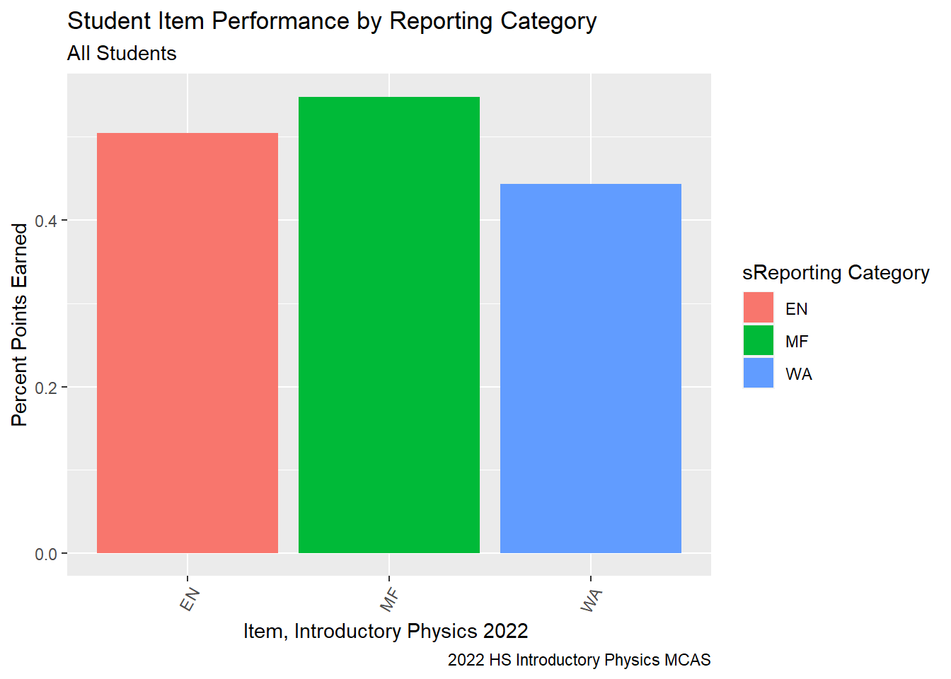
Our second data set, MCAS_G9Science2022_ItemAnalysis is 42 by 9 and consists of 9 variables with information pertaining to the 2022 HS Introductory Physics Item Report. The variables can be broken down into 2 categories:
Details about a given test item: - content Reporting Category (MF (motion and forces) WA (waves), and EN (energy),
Standard from the Massachusetts Curriculum Framework,
Item Description providing the details of what was asked of students.
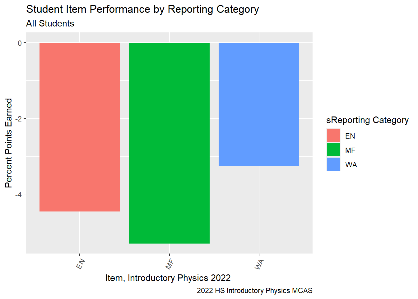
Summary Performance Metrics:
Here you can see the percentage of points earned by students at Rising Tide on an item vs. the percentage of points earned by students in Massachusetts.
I am interested in analyzing the 9th Grade Science Performance. To do this, I will select a subset of our data frame. I selected:
9th Grade and 10th grade students (since a few 10th grade students also took the test)
Scores on the 42 Science Items
Demographic characteristics of the students.
Then I filtered out the 10th grade students who did not take the test
When I compared this data frame to the State reported analysis, the state analysis only contains 68 students. To be able to use the state data, I thus filtered out our 10, 10th grade students and only looked at the performance of the 9th grade students. Notably, my data frame has 69 entries while the state is reporting data on only 68 students. I will have to investigate this further.
Since I will join this data frame with the MCAS_G9Science2022_ItemAnalysis, using sitem as the key, I need to pivot this data set longer.
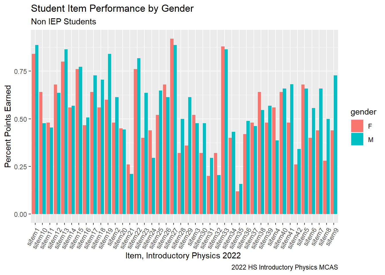
When examining our performance relative to the state by subgroups, it is noteworthy that Rising Tide Female Introductory Physics students on average scored lower relative to their peers in the state and Rising Tide Male Introductory students scored higher on average. This trend is not true for Rising Tide MS science students. When we look at our student’s performance by item and by gender, we can see several questions with a larger disparity in performance by gender.
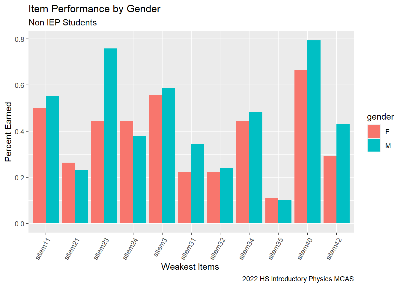
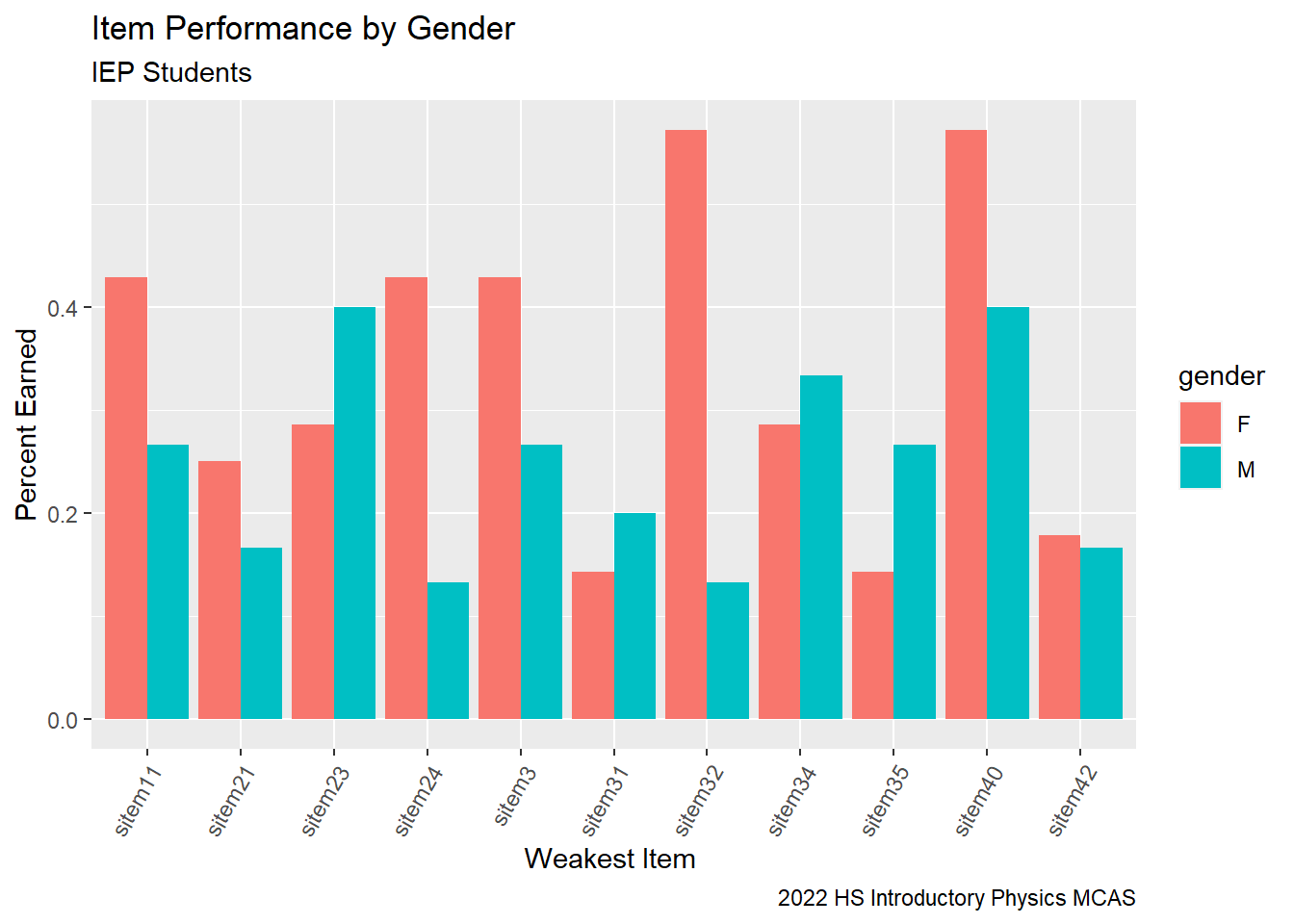
From our students who are not on IEPs, Male students seem to have had more success with questions where they were required to calculate than our female students. Now, we can examine our students on IEPs.
It seems as though we have the opposite trend in our students who are on IEP plans. Perhaps the accommodations and modifications of these plans are more beneficial to female students or perhaps the male students on plans have stronger disabilities.
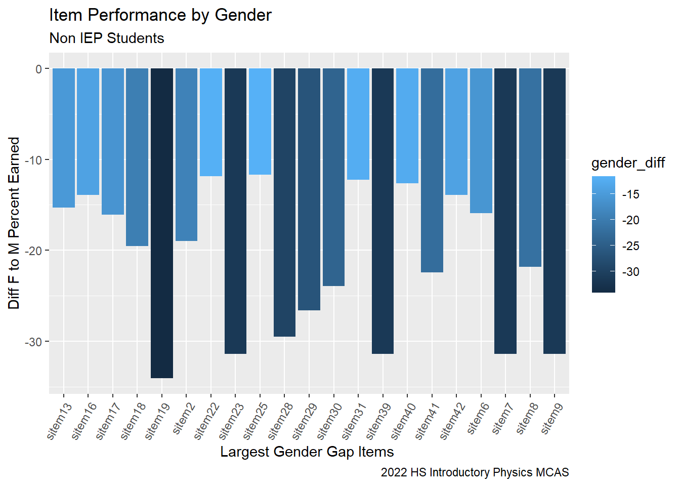
Where is the gender gap the largest? There are many things to examine here and I am running out of time…
Generated by summarytools 1.0.1 (R version 4.2.1) 2022-12-21
Code
G9ScienceGender %>%filter(gender_diff <-10)%>%ggplot(aes(fill = gender_diff , y = gender_diff, x=sitem)) +geom_bar(position="dodge", stat="identity") +labs(subtitle ="Non IEP Students" ,y ="Diff F to M Percent Earned",x="Largest Gender Gap Items ",title ="Item Performance by Gender",caption ="2022 HS Introductory Physics MCAS")+theme(axis.text.x=element_text(angle=60,hjust=1))#+
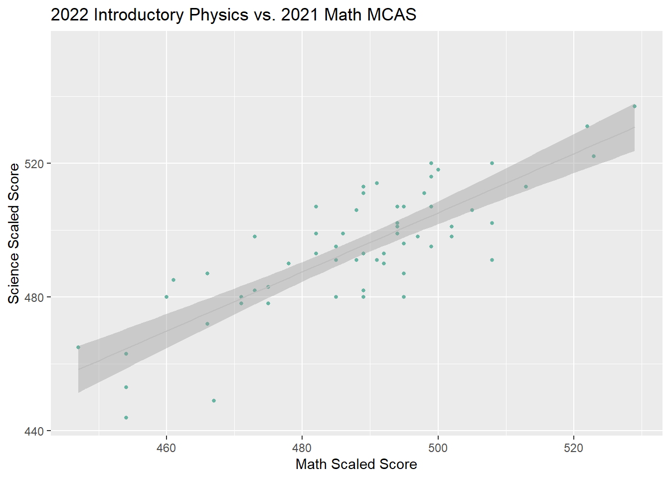
Using Prior Math MCAS result to predict Introductory Physics MCAS Performance. Could we use prior Math MCAS scores to identify students who need extra support for their Science MCAS.
---title: "Challenge 8"author: "Theresa Szczepanski"description: "Joining Data"date: "11/3/2022"format: html: df-print: paged toc: true code-fold: true code-copy: true code-tools: truecategories: - Theresa_Szczepanski - challenge_8 - MCAS_2022 - MCAS_G9Science2022_ItemAnalysis---```{r}#| label: setup#| warning: false#| message: falselibrary(tidyverse)library(ggplot2)library(lubridate)library(readxl)knitr::opts_chunk$set(echo =TRUE, warning=FALSE, message=FALSE)```## Challenge OverviewToday's challenge is to:1) read in multiple data sets, and describe the data set using both words and any supporting information (e.g., tables, etc)2) tidy data (as needed, including sanity checks)3) mutate variables as needed (including sanity checks)4) join two or more data sets and analyze some aspect of the joined data(be sure to only include the category tags for the data you use!)## MCAS_2022.csv ::: panel-tabset### Read in Data Set 1To read in the `MCAS_2022` data, I used the following process:- Filter out Student Names and then Read in the data- Examine the summary- Identify information to filter, mutate, and rename on the read in- note variables that require further investigation::: panel-tabset### Filter, Rename, and Mutate on Read inAfter examining the summary (see tab), I chose to **Filter**:- _SchoolID_ : There are several variables that identify our school, I removed allbut one, `testschoolcode`.- _StudentPrivacy_: I left the `sasid` variable which is a student identifier number,but eliminated all values corresponding to students' names.- `dis`: We are a charter school within our own unique district, therefore any "district level" data is identical to our "school level" data.__Rename__I currently have not renamed variables, but I have a list of variables for which I need to talk with my administration to access a key to understand what they represent.Ideally, after this, I would put - an `E_` before all `ELA` MCAS student performance metric variables- an `M_` before all `Math` MCAS student performance metric variables- an `S_` before all `Science` MCAS student performance metric variables- an `SI_` before all student demographic characteristic identifying variables__Mutate__ I left as __doubles__ - variables that measured scores on specific MCAS items e.g., `mitem1` - variables that measured student growth percentiles (`sgp`) - variables that counted a student's years in the school system or state. Recode to __char__ - variables that are __nominal__, e.g., `town` Refactor as __ord__ - variables that are __ordinal__, e.g., `mperflev`. Recode to __date__ -`dob` using lubridate.```{r}#Filter, rename variables, and mutate values of variables on read-inMCAS_2022<-read_csv("_data/PrivateSpring2022_MCAS_full_preliminary_results_04830305.csv",skip=1)%>%select(-c("sprp_dis", "sprp_sch", "sprp_dis_name", "sprp_sch_name", "sprp_orgtype","schtype", "testschoolname", "yrsindis", "conenr_dis"))%>%#Recode all nominal variables as charactersmutate(testschoolcode =as.character(testschoolcode))%>%# mutate(sasid = as.character(sasid))%>%mutate(highneeds =as.character(highneeds))%>%mutate(lowincome =as.character(lowincome))%>%mutate(title1 =as.character(title1))%>%mutate(ever_EL =as.character(ever_EL))%>%mutate(EL =as.character(EL))%>%mutate(EL_FormerEL =as.character(EL_FormerEL))%>%mutate(FormerEL =as.character(FormerEL))%>%mutate(ELfirstyear =as.character(ELfirstyear))%>%mutate(IEP =as.character(IEP))%>%mutate(plan504 =as.character(plan504))%>%mutate(firstlanguage =as.character(firstlanguage))%>%mutate(nature0fdis =as.character(natureofdis))%>%mutate(spedplacement =as.character(spedplacement))%>%mutate(town =as.character(town))%>%mutate(ssubject =as.character(ssubject))%>%#Recode all ordinal variable as factorsmutate(grade =as.factor(grade))%>%mutate(levelofneed =as.factor(levelofneed))%>%mutate(eperf2 =recode_factor(eperf2,"E"="E","M"="M","PM"="PM","NM"="NM",.ordered =TRUE))%>%mutate(eperflev =recode_factor(eperflev,"E"="E","M"="M","PM"="PM","NM"="NM","DNT"="DNT","ABS"="ABS",.ordered =TRUE))%>%mutate(mperf2 =recode_factor(mperf2,"E"="E","M"="M","PM"="PM","NM"="NM",.ordered =TRUE))%>%mutate(mperflev =recode_factor(mperflev,"E"="E","M"="M","PM"="PM","NM"="NM","INV"="INV","ABS"="ABS",.ordered =TRUE))%>%# The science variables contain a mixture of legacy performance levels and# next generation performance levels which needs to be addressed in the ordering# of these factors.mutate(sperf2 =recode_factor(sperf2,"E"="E","M"="M","PM"="PM","NM"="NM",.ordered =TRUE))%>%mutate(sperflev =recode_factor(sperflev,"E"="E","M"="M","PM"="PM","NM"="NM","INV"="INV","ABS"="ABS",.ordered =TRUE))%>%#recode DOB using lubridatemutate(dob =mdy(dob,quiet =FALSE,tz =NULL,locale =Sys.getlocale("LC_TIME"),truncated =0))view(MCAS_2022)MCAS_2022```### Post Read In Summary```{r}# examine the summary to decide how to best set up our data frameprint(summarytools::dfSummary(MCAS_2022,varnumbers =FALSE,plain.ascii =FALSE,style ="grid",graph.magnif =0.70,valid.col =FALSE),method ='render',table.classes ='table-condensed')```:::### Read in Data Set 2To read in `MCAS_G9Science2022_ItemAnalysis`, I:- Selected only the 9th Grade Physics Item Report- Deleted an extra column from a cell merge- refactored the `sitem` variable to prepare to join this data set to the Student performance data set.- Added an s to the column names as a reminder that all of these columns relate to the Science exam.```{r}library(readxl)# G9 Science Item analysisMCAS_G9Science2022_ItemAnalysis<-read_excel("_data/2022MCASDepartmentalAnalysis.xlsx", sheet ="SG9Physics", skip =1, col_names=c("sitem", "sType", "sReporting Category", "sStandard", "sItem Desc", "delete", "sItem Possible Points","RT Percent Points", "State Percent Points", "RT-State Diff")) %>%select(!contains("delete"))%>%filter(str_detect(sStandard, "HS"))%>%mutate("sitem"=as.character(sitem))#view(MCAS_G9Science2022_ItemAnalysis)# use string r to fix the item #MCAS_G9Science2022_ItemAnalysis<-separate(MCAS_G9Science2022_ItemAnalysis, sitem, c("sitem", "delete"))%>%select(!contains("delete"))%>%mutate(sitem =str_c("sitem", sitem))MCAS_G9Science2022_ItemAnalysisview(MCAS_G9Science2022_ItemAnalysis)```### Narrative SummaryFrom our `MCAS_2022` data frame summary, we can see that this data setcontains performance results from 495 students from [Rising Tide Charter Public School](https://risingtide.org/) on the Spring 2022 [Massachusetts Comprehensive Assessment System (MCAS)](https://www.doe.mass.edu/mcas/default.html)tests.For each student, there are values reported for 256 different variables which consist of information from four broad categories- *Demographic characteristics* of the students themselves (e.g., race, gender, date of birth, town, grade level, years in school, years in Massachusetts, and low income, title1, IEP, 504m and EL status ). - *Key assessment features* including subject, test format, andaccommodations provided - *Performance metrics*: This includes a students score on individual item strands, e.g.,`mitem1`-`mitem42`. Our second data set, `MCAS_G9Science2022_ItemAnalysis` is 42 by 9 and consists of 9 variables with information pertaining to the 2022 [HS Introductory Physics Item Report](https://profiles.doe.mass.edu/mcas/mcasitems2.aspx?grade=HS&subjectcode=PHY&linkid=23&orgcode=04830000&fycode=2022&orgtypecode=5&). The variables can be broken down into 2 categories: Details about a given test item: - content `Reporting Category` (MF (motion and forces)WA (waves), and EN (energy), - `Standard` from the Massachusetts Curriculum Framework, - `Item Description` providing the details of what was asked of students.Summary Performance Metrics:- Here you can see the percentage of points earned by students at Rising Tide on an itemvs. the percentage of points earned by students in Massachusetts.### Tidy Data to Prep for JoinI am interested in analyzing the 9th Grade Science Performance. To do this, I will select a subset of our data frame. I selected:- 9th Grade and 10th grade students (since a few 10th grade students also took the test)- Scores on the 42 Science Items- Demographic characteristics of the students.Then I filtered out the 10th grade students who did not take the test```{r}G9ScienceMCAS_2022 <-select(MCAS_2022, contains("sitem"), gender, grade, yrsinsch, race, IEP, `plan504`, sattempt)%>%filter((grade ==9) & sattempt !="N")G9ScienceMCAS_2022<-select(G9ScienceMCAS_2022, !(contains("43")|contains("44")|contains("45")))view(G9ScienceMCAS_2022)G9ScienceMCAS_2022```When I compared this data frame to the State reported analysis, the state analysis only contains 68 students. To be able to use the state data, I thus filtered out our 10, 10th grade students and only looked at the performance of the 9th grade students. Notably, my data frame has 69 entries while the state is reporting data on only 68 students. I will have to investigate this further.Since I will join this data frame with the `MCAS_G9Science2022_ItemAnalysis`, using `sitem` as the key, I need to pivot this data set longer.```{r}G9ScienceMCAS_2022<-pivot_longer(G9ScienceMCAS_2022, contains("sitem"), names_to ="sitem", values_to ="sitem_score")view(G9ScienceMCAS_2022)G9ScienceMCAS_2022```As expected, we now have 42 X 69 = 2898 rows. ### Join DataNow, we should be ready to join our data sets using `sitem` as the key. We should have a 2,898 by (9 + 8) = 2,898 by 17 data frame.```{r}G9Science_StudentItem <- G9ScienceMCAS_2022 %>%left_join(MCAS_G9Science2022_ItemAnalysis, "sitem")%>%view(G9Science_StudentItem)G9Science_StudentItem```As expected, we now have a 2,898 \times 17 data frame.### Analysis of Joined DataWhen examining our performance relative to the [state by subgroups](https://profiles.doe.mass.edu/mcas/subgroups2.aspx?linkid=25&orgcode=04830305&fycode=2022&orgtypecode=6&), it is noteworthy that Rising Tide Female Introductory Physics students on average scored lower relative to their peers in the state and Rising Tide Male Introductory students scored higher on average. This trend is not true for Rising Tide MS science students. When we look at our student's performance by item and by gender, we can see several questions with a larger disparity in performance by gender.```{r}G9Science_Gender<-G9Science_StudentItem%>%select(gender, sitem, sitem_score, `sItem Desc`, `sItem Possible Points`, `State Percent Points`, IEP)%>%group_by(gender, sitem)%>%summarise(sitem_percent =sum(sitem_score, na.rm=TRUE)/sum(`sItem Possible Points`))ggplot(G9Science_Gender, aes(fill=gender, y=sitem_percent, x=sitem)) +geom_bar(position="dodge", stat="identity") +labs(subtitle ="Non IEP Students" ,y ="Percent Points Earned",x="Item, Introductory Physics 2022 ",title ="Student Item Performance by Gender",caption ="2022 HS Introductory Physics MCAS")+theme(axis.text.x=element_text(angle=60,hjust=1))```Now let's examine the items where students had the weakest performance relative to the state.```{r}# G9 Science Calculate Non IEP Gender AnalysisG9Science_Gender_NonIEP<-G9Science_StudentItem%>%select(gender, sitem, sitem_score, `sItem Desc`, `sItem Possible Points`, `State Percent Points`, IEP, `RT-State Diff`)%>%filter(`RT-State Diff`<=-10)%>%filter(IEP ==0)%>%group_by(gender, sitem) %>%summarise(gender_percent =sum(sitem_score, na.rm=TRUE)/sum(`sItem Possible Points`))G9Science_Gender_NonIEP# Grouped bar Chart Calculate ItemsG9Science_Gender_NonIEP%>%ggplot(aes(fill=gender, y=gender_percent, x=sitem)) +geom_bar(position="dodge", stat="identity") +labs(subtitle ="Non IEP Students" ,y ="Percent Earned",x="Weakest Items ",title ="Item Performance by Gender",caption ="2022 HS Introductory Physics MCAS")+theme(axis.text.x=element_text(angle=60,hjust=1))#+#coord_flip()```From our students who are not on IEPs, Male students seem to have had more success with questions where they were required to calculate than our female students. Now, we can examine our students on IEPs.```{r}# G9 Science Calculate IEP Gender AnalysisG9Science_Gender_IEP<-G9Science_StudentItem%>%select(gender, sitem, sitem_score, `sItem Desc`, `sItem Possible Points`, `State Percent Points`, IEP, `RT-State Diff`)%>%filter(`RT-State Diff`<=-10)%>%filter(IEP !=0)%>%group_by(gender, sitem) %>%group_by(gender, sitem) %>%summarise(gender_percent =sum(sitem_score, na.rm=TRUE)/sum(`sItem Possible Points`))G9Science_Gender_IEPG9Science_Gender_IEP%>%ggplot(aes(fill=gender, y=gender_percent, x=sitem)) +geom_bar(position="dodge", stat="identity") +labs(subtitle ="IEP Students" ,y ="Percent Earned",x="Weakest Item ",title ="Item Performance by Gender",caption ="2022 HS Introductory Physics MCAS")+theme(axis.text.x=element_text(angle=60,hjust=1))#+#coord_flip()```It seems as though we have the opposite trend in our students who are on IEP plans. Perhaps the accommodations and modifications of these plans are more beneficial to female students or perhaps the male students on plans have stronger disabilities.Where is the gender gap the largest? There are many things to examine here and I am running out of time...```{r}G9Science_Male_NonIEP<-G9Science_StudentItem%>%select(gender, sitem, sitem_score, `sItem Desc`, `sItem Possible Points`, `State Percent Points`, IEP, `RT-State Diff`)%>%filter(gender =="M")%>%filter(IEP ==0)%>%group_by(sitem) %>%summarise(male_percent =sum(sitem_score, na.rm=TRUE)/sum(`sItem Possible Points`))G9Science_Female_NonIEP<-G9Science_StudentItem%>%select(gender, sitem, sitem_score, `sItem Desc`, `sItem Possible Points`, `State Percent Points`, IEP, `RT-State Diff`)%>%filter(gender =="F")%>%filter(IEP ==0)%>%group_by(sitem) %>%summarise(female_percent =sum(sitem_score, na.rm=TRUE)/sum(`sItem Possible Points`))G9ScienceGender<-G9Science_Female_NonIEP%>%left_join(G9Science_Male_NonIEP, "sitem")%>%mutate(gender_diff =100*(female_percent - male_percent))# pivot_longer(female_percent, male_percent, names_to = gender, values_to = item_percent)G9ScienceGenderprint(summarytools::dfSummary(G9ScienceGender,varnumbers =FALSE,plain.ascii =FALSE,style ="grid",graph.magnif =0.70,valid.col =FALSE),method ='render',table.classes ='table-condensed')G9ScienceGender %>%filter(gender_diff <-10)%>%ggplot(aes(fill = gender_diff , y = gender_diff, x=sitem)) +geom_bar(position="dodge", stat="identity") +labs(subtitle ="Non IEP Students" ,y ="Diff F to M Percent Earned",x="Largest Gender Gap Items ",title ="Item Performance by Gender",caption ="2022 HS Introductory Physics MCAS")+theme(axis.text.x=element_text(angle=60,hjust=1))#+```Using Prior Math MCAS result to predict Introductory Physics MCAS Performance. Could we use prior Math MCAS scores to identify students who need extra support for their Science MCAS.```{r}#view(MCAS_2022) MCAS_subset<-select(MCAS_2022, sscaleds, gender, grade, yrsinsch, , IEP, `plan504`, sattempt, mattempt,mscaleds2021 )%>%filter((grade ==9) & sattempt !="N")ggplot(MCAS_subset, aes(x=mscaleds2021, y=sscaleds, color=gender)) +geom_point(size =1, color="#69b3a2")+geom_smooth(method="lm",color="grey", size =.5 )+labs(title ="2022 Introductory Physics vs. 2021 Math MCAS", y ="Science Scaled Score",x ="Math Scaled Score")# +#facet_wrap(vars(gender))#theme_minimal()```Science Performance by Reporting Category: Should teachers review a given unit more closely.```{r}G9Science_Desc<-G9Science_StudentItem%>%select(gender, sitem, sitem_score, `sReporting Category`, `sItem Possible Points`, `State Percent Points`, `RT-State Diff`, IEP)%>%group_by(`sReporting Category`)%>%summarise(desc_percent =sum(sitem_score, na.rm=TRUE)/sum(`sItem Possible Points`))ggplot(G9Science_Desc, aes(fill =`sReporting Category`, y=desc_percent, x=`sReporting Category`)) +geom_bar(position="dodge", stat="identity") +labs(subtitle ="All Students" ,y ="Percent Points Earned",x="Item, Introductory Physics 2022 ",title ="Student Item Performance by Reporting Category",caption ="2022 HS Introductory Physics MCAS")+theme(axis.text.x=element_text(angle=60,hjust=1))```RT State Difference by Reporting Category```{r}G9Science_StateDiff<-G9Science_StudentItem%>%select(gender, sitem, sitem_score, `sReporting Category`, `sItem Possible Points`, `State Percent Points`, `RT-State Diff`, IEP)%>%group_by(`sReporting Category`)%>%summarise(avg_RT_State_Diff =mean(`RT-State Diff`, na.rm=TRUE))ggplot(G9Science_StateDiff, aes(fill =`sReporting Category`, y=`avg_RT_State_Diff`, x=`sReporting Category`)) +geom_bar(position="dodge", stat="identity") +labs(subtitle ="All Students" ,y ="Percent Points Earned",x="Item, Introductory Physics 2022 ",title ="Student Item Performance by Reporting Category",caption ="2022 HS Introductory Physics MCAS")+theme(axis.text.x=element_text(angle=60,hjust=1))``````{r}G9Science_Calculate<-G9Science_StudentItem%>%select(gender, sitem, sitem_score, `sItem Desc`, `sReporting Category`, `sItem Possible Points`, `State Percent Points`, `RT-State Diff`, IEP)%>%filter(str_detect(`sItem Desc`, "calculate|Calculate")) #%>%#print( summarise(avg_RT_State_Diff = mean(`RT-State Diff`, na.rm=TRUE)))#mean(`RT-State Diff`, na.rm=TRUE)#G9Science_Calculate#%>%# ggplot(aes(fill = `sReporting Category`, y=`avg_RT_State_Diff`, x=`sReporting Category`)) +# geom_bar(position="dodge", stat="identity") +# group_by(`sReporting Category`)%>%# summarise(avg_RT_State_Diff = mean(`RT-State Diff`, na.rm=TRUE))# # ggplot(G9Science_StateDiff, aes(fill = `sReporting Category`, y=`avg_RT_State_Diff`, x=`sReporting Category`)) +# geom_bar(position="dodge", stat="identity") +# labs(subtitle ="All Students" ,# y = "Percent Points Earned",# x= "Item, Introductory Physics 2022 ",# title = "Student Item Performance by Reporting Category",# caption = "2022 HS Introductory Physics MCAS")+# theme(axis.text.x=element_text(angle=60,hjust=1))```:::