For each student, there are values reported for 256 different variables which consist of information from four broad categories
Demographic characteristics of the students themselves (e.g., race, gender, date of birth, town, grade level, years in school, years in Massachusetts, and low income, title1, IEP, 504, and EL status ).
Key assessment features including subject, test format, and accommodations provided
Performance metrics: This includes a student’s score on individual item strands, e.g.,mitem1-mitem42.
See the MCAS_2022 data frame summary and codebook in the appendix for further details.
The second data set, MCAS_G9Sci2022_Item, is 42 by 9 and consists of 9 variables with information pertaining to the 42 questions on the 2022 HS Introductory Physics Item Report. The variables can be broken down into 2 categories:
Details about the content of a given test item:
This includes the content Reporting Category (MF (motion and forces) WA (waves), and EN (energy), the Standard from the 2016 STE Massachusetts Curriculum Framework, the Item Description providing the details of what specifically was asked of students, and the points available for a given question, sitem Possible Points.
Summary Performance Metrics:
For each item, the state reports the percentage of points earned by students at Rising Tide, RT Percent Points, the percentage of available points earned by students in the state, State Percent Points, and the difference between the percentage of points earned by Rising Tide students and the percentage of points earned by students in the state, RT-State Diff.
Lastly, CU306 Disability, is a 3 X 5 dataframe consisting of summary performance data by sItem Reporting Category for students with disabilities; most importantly including RT Percent Points and State Percent Points.
When considering our student performance data, we hope to address the following broad questions:
What adjustments (if any) should be made at the Tier 1 level, i.e., curricular adjustments for all students?
What would be the most beneficial areas of focus for a targeted intervention course for students struggling to meet or exceed performance expectations?
Are there notable differences in student performance for students with and without disabilities?
Function Library
To read in, tidy, and join our data frames for each content area we will use the following functions. This still needs to be made more adaptable to include Math and ELA.
#Filter, rename variables, and mutate values of variables on read-inMCAS_2022<-read_csv("_data/PrivateSpring2022_MCAS_full_preliminary_results_04830305.csv",skip=1)%>%select(-c("sprp_dis", "sprp_sch", "sprp_dis_name", "sprp_sch_name", "sprp_orgtype","schtype", "testschoolname", "yrsindis", "conenr_dis"))%>%#Recode all nominal variables as charactersmutate(testschoolcode =as.character(testschoolcode))%>%# mutate(sasid = as.character(sasid))%>%mutate(highneeds =as.character(highneeds))%>%mutate(lowincome =as.character(lowincome))%>%mutate(title1 =as.character(title1))%>%mutate(ever_EL =as.character(ever_EL))%>%mutate(EL =as.character(EL))%>%mutate(EL_FormerEL =as.character(EL_FormerEL))%>%mutate(FormerEL =as.character(FormerEL))%>%mutate(ELfirstyear =as.character(ELfirstyear))%>%mutate(IEP =as.character(IEP))%>%mutate(plan504 =as.character(plan504))%>%mutate(firstlanguage =as.character(firstlanguage))%>%mutate(nature0fdis =as.character(natureofdis))%>%mutate(spedplacement =as.character(spedplacement))%>%mutate(town =as.character(town))%>%mutate(ssubject =as.character(ssubject))%>%#Recode all ordinal variable as factorsmutate(grade =as.factor(grade))%>%mutate(levelofneed =as.factor(levelofneed))%>%mutate(eperf2 =recode_factor(eperf2,"E"="E","M"="M","PM"="PM","NM"="NM",.ordered =TRUE))%>%mutate(eperflev =recode_factor(eperflev,"E"="E","M"="M","PM"="PM","NM"="NM","DNT"="DNT","ABS"="ABS",.ordered =TRUE))%>%mutate(mperf2 =recode_factor(mperf2,"E"="E","M"="M","PM"="PM","NM"="NM",.ordered =TRUE))%>%mutate(mperflev =recode_factor(mperflev,"E"="E","M"="M","PM"="PM","NM"="NM","INV"="INV","ABS"="ABS",.ordered =TRUE))%>%# The science variables contain a mixture of legacy performance levels and# next generation performance levels which needs to be addressed in the ordering# of these factors.mutate(sperf2 =recode_factor(sperf2,"E"="E","M"="M","PM"="PM","NM"="NM",.ordered =TRUE))%>%mutate(sperflev =recode_factor(sperflev,"E"="E","M"="M","PM"="PM","NM"="NM","INV"="INV","ABS"="ABS",.ordered =TRUE))%>%#recode DOB using lubridatemutate(dob =mdy(dob,quiet =FALSE,tz =NULL,locale =Sys.getlocale("LC_TIME"),truncated =0))#view(MCAS_2022)MCAS_2022
After examining the summary (see appendix), I chose to
Filter:
SchoolID : There are several variables that identify our school, I removed all but one, testschoolcode.
StudentPrivacy: I left the sasid variable which is a student identifier number, but eliminated all values corresponding to students’ names.
dis: We are a charter school within our own unique district, therefore any “district level” data is identical to our “school level” data.
Rename
I currently have not renamed variables, but there are some trends to note:
an e before most ELA MCAS student item performance metric variables
an m before most Math MCAS student item performance metric variables
an s before most Science MCAS student item performance metric variables
Mutate
I left as doubles
variables that measured scores on specific MCAS items e.g., mitem1
variables that measured student growth percentiles (sgp)
variables that counted a student’s years in the school system or state.
Recode to char
variables that are nominal but have numeric values, e.g., town
When I compared this data frame to the State reported analysis, the state analysis only contains 68 students. Notably, my data frame has 69 entries while the state is reporting data on only 68 students. I will have to investigate this further.
Since I will join this data frame with the MCAS_G9Sci2022_Item, using sitem as the key, I need to pivot this data set longer.
Now, we should be ready to join our data sets using sitem as the key. We should have a 2,898 by (10 + 8) = 2,898 by 18 data frame. We will also check our raw data against the performance data reported by the state in the item report by calculating percent_earned by Rising Tide students and comparing it to the figure RT Percent Points and storing the difference in earned_diff
As expected, we now have a 2,898 X 18 data frame and the earned_diff values all round to 0.
G9 Science Performance Analysis
When considering our student performance data, we hope to address the following broad questions:
What adjustments (if any) should be made at the Tier 1 level, i.e., curricular adjustments for all students?
What would be the most beneficial areas of focus for a targeted intervention course for students struggling to meet or exceed performance expectations?
Are there notable differences in student performance for students with and without disabilities?
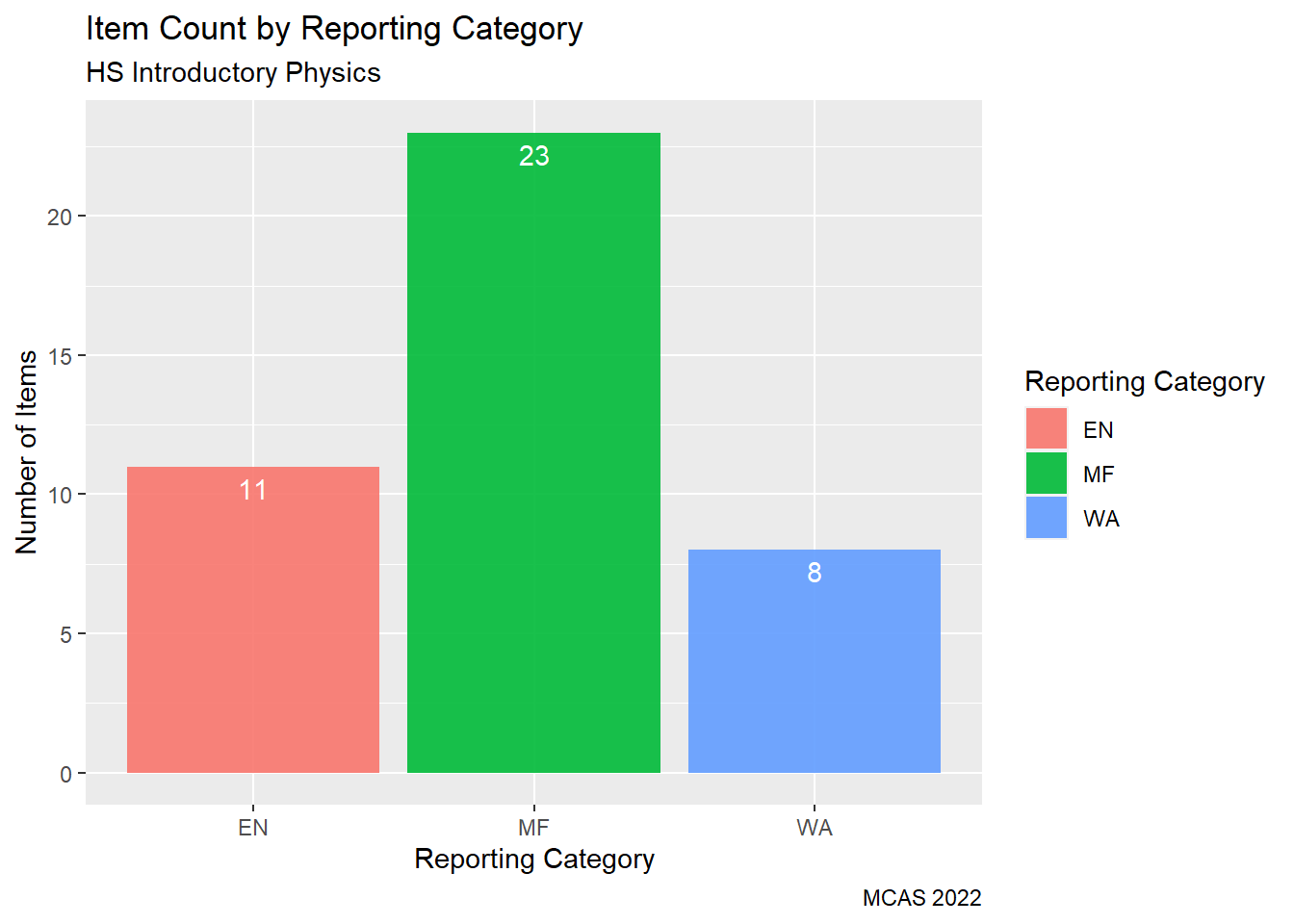
What reporting categories were emphasized by the state?
We can see from our summary,that 50% of the exam points (30 of the available 60) come from questions from the Motion and Forces reporting category and 23 of the 42 questions were from this category.
ggplot(G9Science_Cat_Total, aes(x=`Reporting Category`, fill =`Reporting Category`))+geom_bar( alpha=0.9) +labs(title ="Item Count by Reporting Category",subtitle ="HS Introductory Physics",caption ="MCAS 2022", y ="Number of Items", x ="Reporting Category") +geom_text(aes(label = ..count..), stat ="count", vjust =1.5, colour ="white")
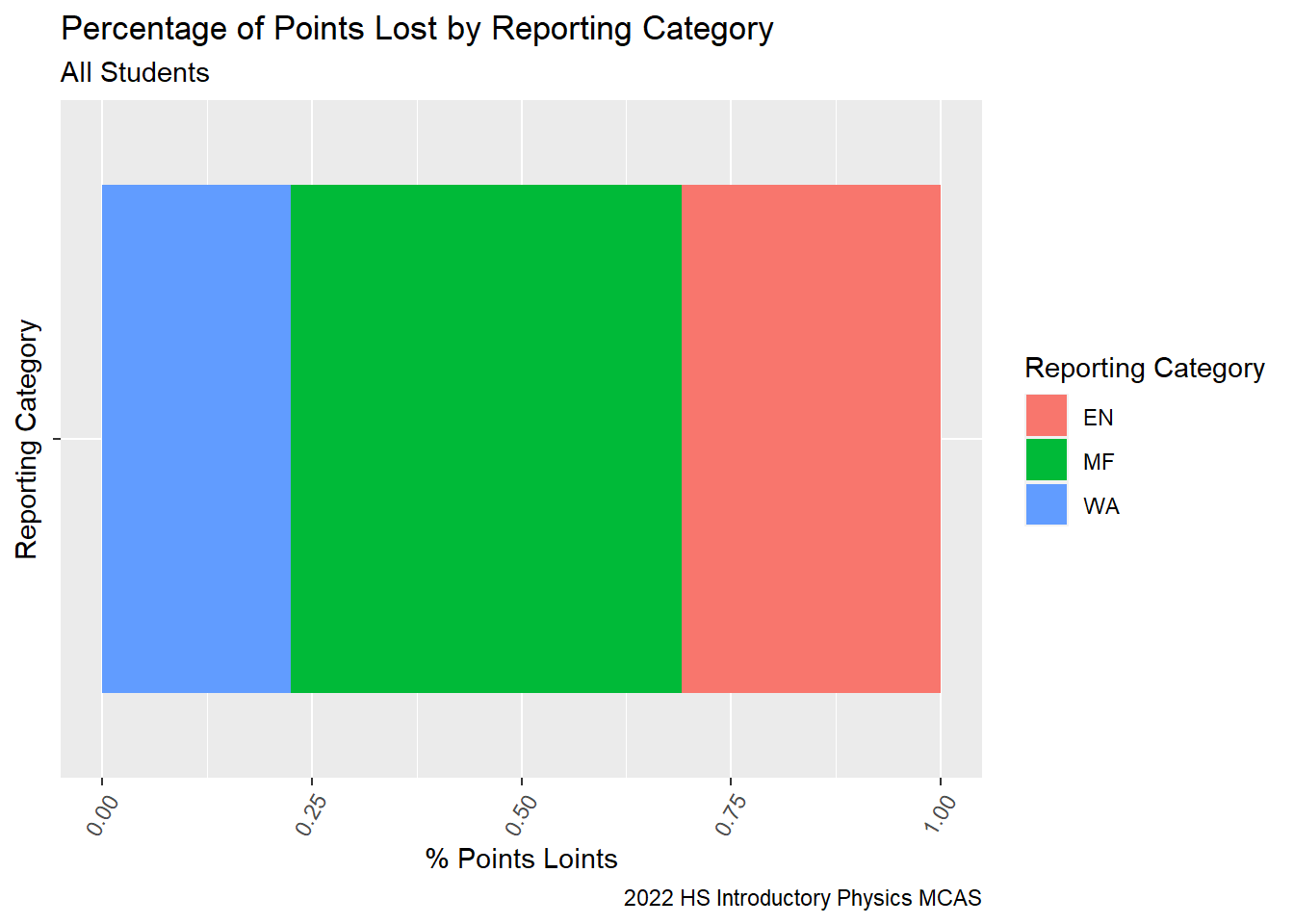
Where did RT students lose most of their points? Students lost the largest proportion of points in the Motion and Forces category, which was the Reporting Category for 50% of the points on the exam. The points lost by Rising Tide students seem to be proportional to the number of points available for each category.
Code
G9Science_Cat_Loss<-G9Science_StudentItem%>%select(`sitem`, `Reporting Category`, `item Possible Points`, `sitem_score`)%>%group_by(`Reporting Category`)%>%summarise(sum_points_lost =sum(`item Possible Points`-`sitem_score`, na.rm=TRUE))
Code
G9Science_Percent_Loss<-G9Science_StudentItem%>%select(`sitem`, `Reporting Category`, `item Possible Points`, `sitem_score`)%>%mutate(`points_lost`=`item Possible Points`-`sitem_score`)%>%#ggplot(df, aes(x='', fill=option)) + geom_bar(position = "fill") ggplot( aes(x='',fill =`Reporting Category`, y =`points_lost`)) +geom_bar(position="fill", stat ="identity") +coord_flip()+labs(subtitle ="All Students" ,y ="% Points Loints",x="Reporting Category",title ="Percentage of Points Lost by Reporting Category",caption ="2022 HS Introductory Physics MCAS")+theme(axis.text.x=element_text(angle=60,hjust=1))G9Science_Percent_Loss
Code
#
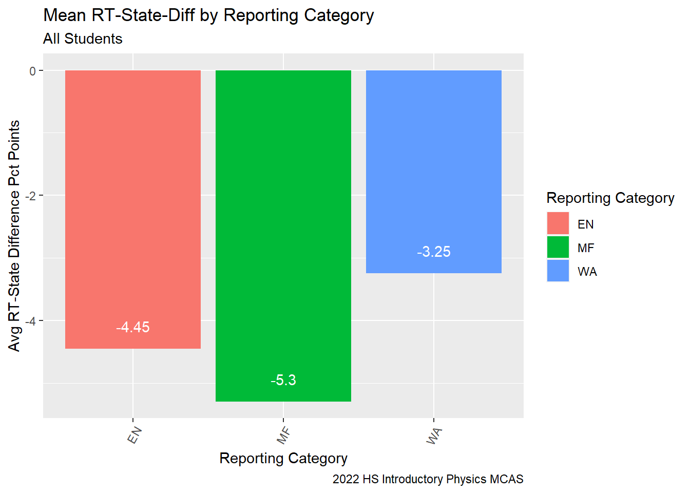
Did Rising Tide students’ performance relative to the state vary by content reporting categories?
Code
#Need to use CU306 and not take average of percentages...but percent of available points# G9Science_Cat_Total%>%# group_by(`Reporting Category`)%>%# summarise(available_points = sum(`item Possible Points`, na.rm=TRUE),# RT_percent_points = round(mean(`RT Percent Points`, na.rm = TRUE),2),# State_percent_points = round(mean(`State Percent Points`, na.rm = TRUE),2))%>%# pivot_longer(contains("percent"), names_to = "Group", values_to = "percent_points")%>%# ggplot( aes(fill = `Group`, y=`percent_points`, x=`Reporting Category`)) +# geom_bar(position="dodge", stat="identity") +# labs(subtitle ="All Students" ,# y = "Mean % Points",# x= "Reporting Category",# title = "Percent Points Earned by Reporting Category",# caption = "2022 HS Introductory Physics MCAS")+# theme(axis.text.x=element_text(angle=60,hjust=1))+# geom_text(aes(label = `percent_points`), vjust = 1.5, colour = "white", position = position_dodge(.9))
As we can see from our table, on average, our students earned fewer points relative to their peers in the state on items across all three reporting categories.
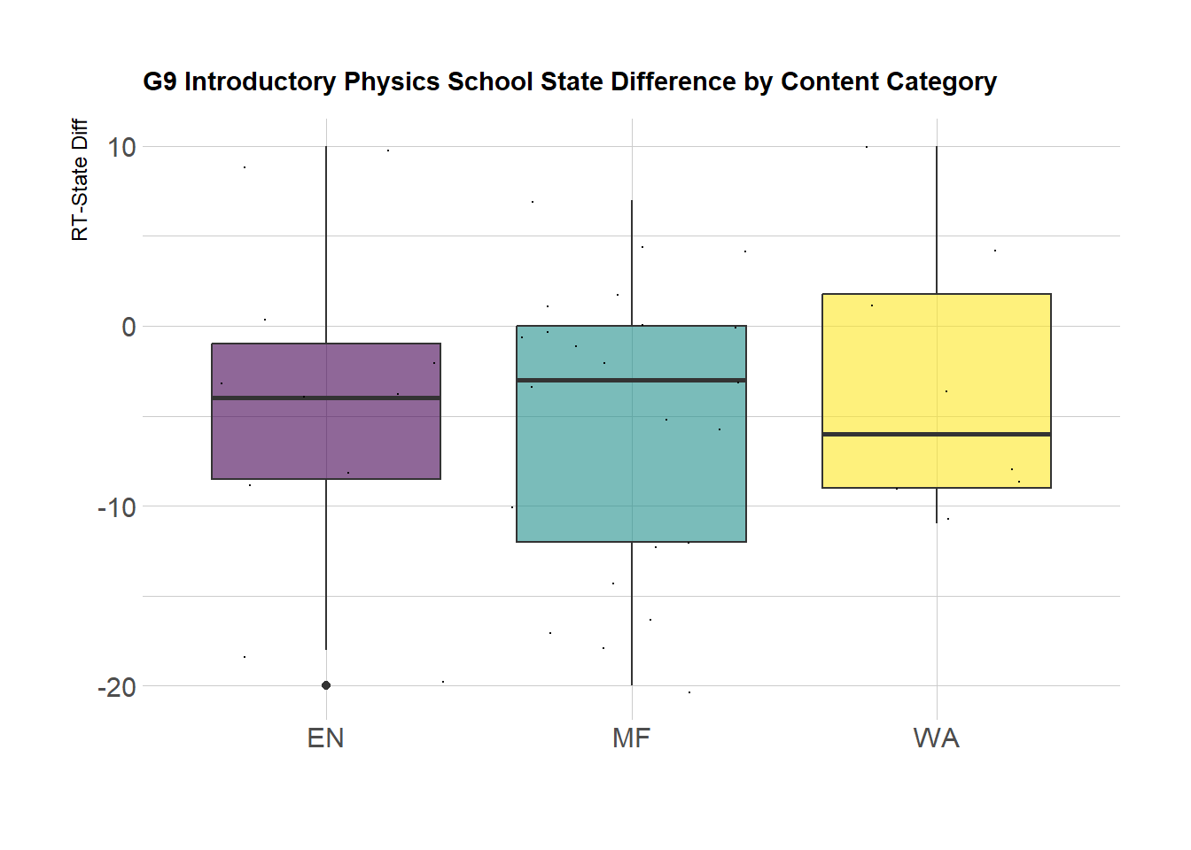
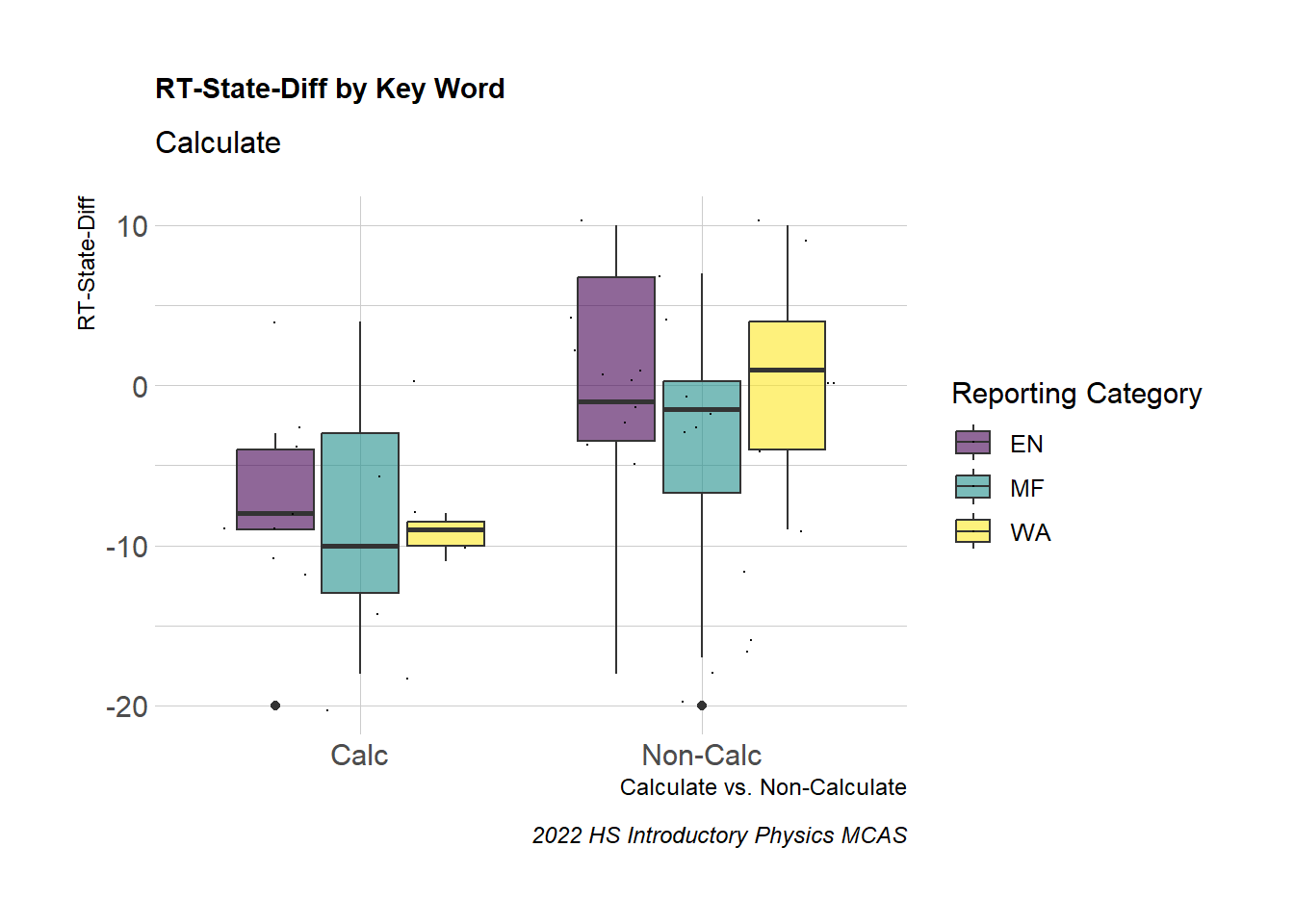
Here we see the distribution of RT-State Diff (difference between the percentage of points earned on a given item by Rising Tide students and percentage of points earned on the same item by their peers in the State) by reporting categor. We can see generally that Motion and Forces seems to have the highest variability. It would be worth looking at the specific question strands with the Physics Teachers. (It would be helpful to add item labels to the dots)
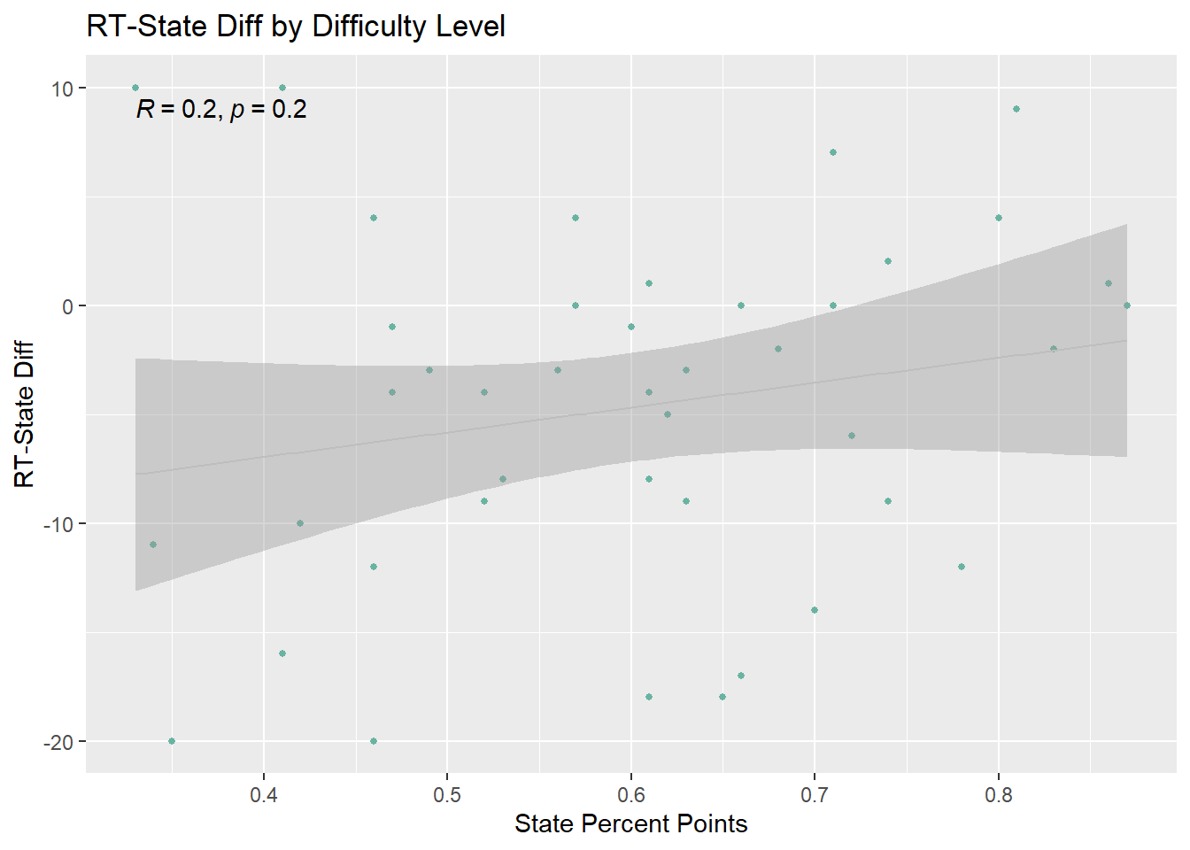
Can differences in Rising Tide student performance on an item and State performance on an item be explained by the difficulty level of an item?
When considering RT-State Diff against State Percent Points this does not seem to generally be the case. Although the regression line shows RT-State Diff more likely to be negative on items where students in the State earned fewer points; the p-value is not significant.
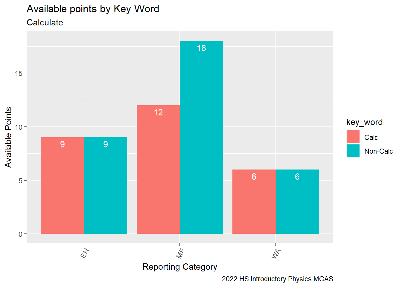
When scanning the item Desc entries, there are several questions containing the word “Calculate” in their description. How much is calculation emphasized on this exam and how did Rising Tide students perform relative to their peers in the state on items containing “calculate” in their description?
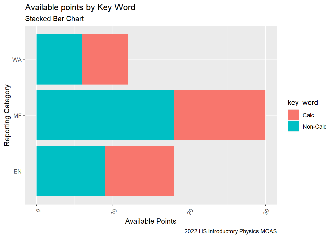
Now, we can see that by the Waves and Energy categories, half of the available points come from questions with calculate and half do not. In the Motion and Forces category, 40% of points are associated with questions that ask students to “calculate”.
G9Science_Calc_PointsAvail_Stacked <- G9Science_Calc%>%ggplot(aes(fill=key_word, y =`item Possible Points`, x=`Reporting Category`)) +geom_bar(position="stack", stat="identity")+labs(subtitle ="Stacked Bar Chart",y ="Available Points",x="Reporting Category",title ="Available points by Key Word",caption ="2022 HS Introductory Physics MCAS")+theme(axis.text.x=element_text(angle=60,hjust=1))+coord_flip() G9Science_Calc_PointsAvail_Stacked
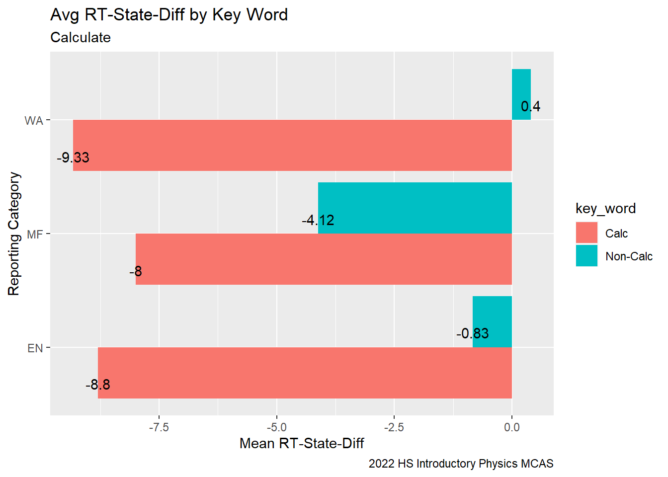
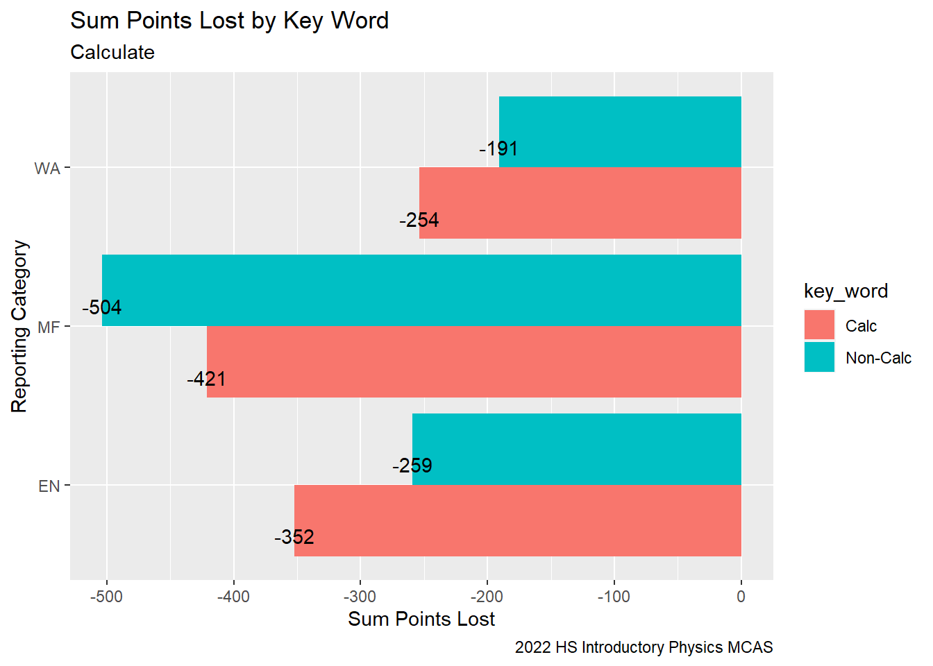
When we compare the mean RT-State Diff for items containing the word “calculate” in their description vs. items that do not, we can see that across all of the Reporting Categories, Rising Tide students performed significantly weaker relative to their peers on questions that asked them to “calculate”.
Here we can see the distribution of RT-State Diff by item, Reporting Category and disparity in the RT-State Diff when we consider the term “Calculate”.
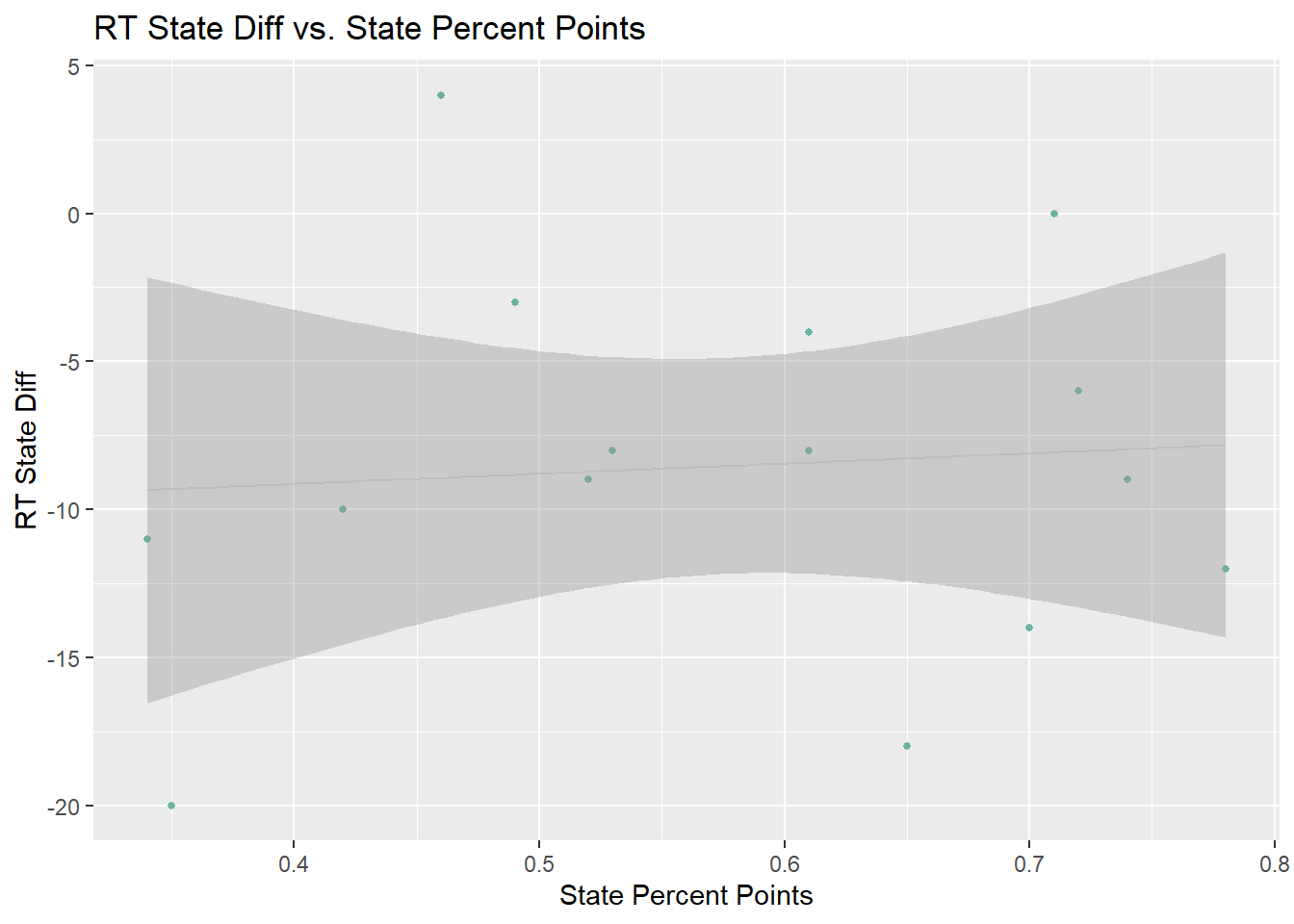
Did RT students perform worse relative to their peers in the state on more “challenging” calculation items? If we consider the difficulty of items containing the word calculate for students as reflected in the state-wide performance (State Percent Points) for a given item, the gap between Rising Tide students’ performance to their peers in the state RT-State Diff does not seem to increase with the difficulty .
Code
view(G9Science_Calc)G9Science_Calc_Dot<- G9Science_Calc%>%select(`State Percent Points`, `RT-State Diff`, `key_word`)%>%filter(key_word =="Calc")%>%ggplot( aes(x=`State Percent Points`, y=`RT-State Diff`)) +geom_point(size =1, color="#69b3a2")+geom_smooth(method="lm",color="grey", size =.5 )+labs(title ="RT State Diff vs. State Percent Points", y ="RT State Diff",x ="State Percent Points")#+ face(vars())G9Science_Calc_Dot
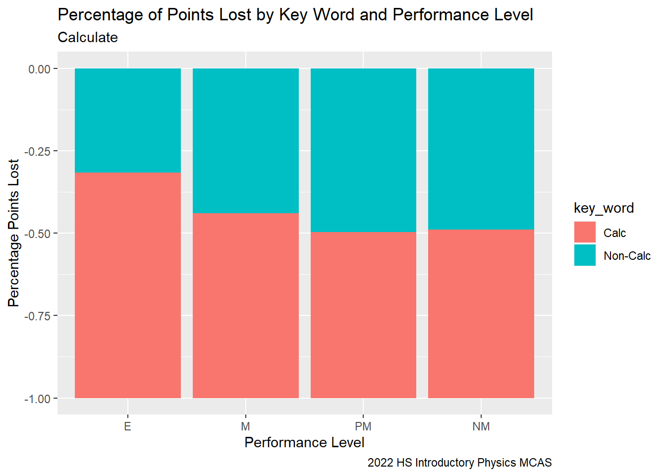
Is the “calculation gap” consistent across performance levels?
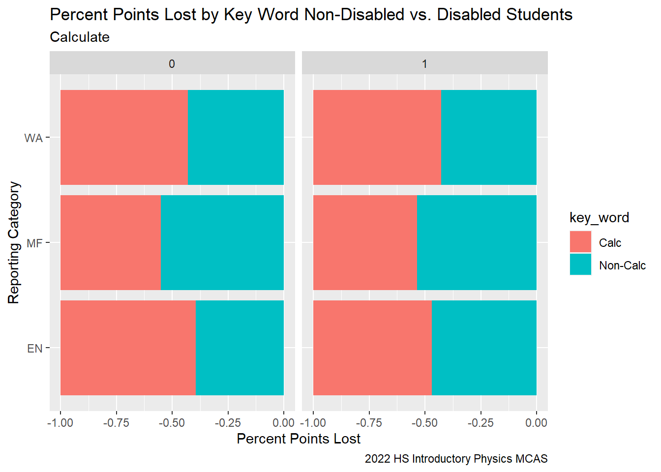
Here we can see that students with a higher performance level, lost a higher proportion of their points on questions involving “Calculate”. I.e., the higher a student’s performance level, the higher percentage of their points were lost to items asking them to “calculate”. This suggests, in the general classroom, to raise student performance, students should spend a higher proportion of time on calculation based activities.
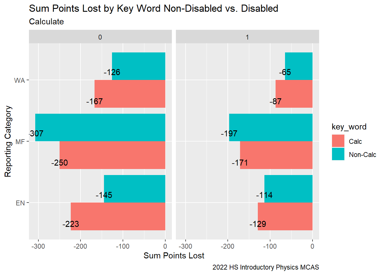
We can see from our CU306 reports, that our students with disabilities performed better relative to their peers in the state RT-State Diff across all Reporting Categories, while our non-disabled students performed worse relative to their peers in the state across all Reporting Categories.
When we examine the points lost by reporting category and disability status, there does not seem to be a difference in performance between disabled and non-disabled students.
Code
G9Sci_StudentCalcDis<-G9Science_StudentItem%>%select(gender, sitem, sitem_score, `item Desc`, `item Possible Points`, `State Percent Points`, IEP, `RT-State Diff`, `Reporting Category`, `sperflev`)%>%mutate( key_word =case_when(!str_detect(`item Desc`, "calculate|Calculate") ~"Non-Calc",str_detect(`item Desc`, "calculate|Calculate") ~"Calc"))%>%group_by(`Reporting Category`, `key_word`, `IEP`)%>%summarise(total_points_lost =sum(`sitem_score`-`item Possible Points`, na.rm =TRUE))%>%ggplot(aes(fill=`key_word`, y=total_points_lost, x=`Reporting Category`)) +geom_bar(position="dodge", stat="identity")+facet_wrap(vars(IEP))+coord_flip()+labs(subtitle ="Calculate" ,y ="Sum Points Lost",x="Reporting Category",title ="Sum Points Lost by Key Word Non-Disabled vs. Disabled",caption ="2022 HS Introductory Physics MCAS")+geom_text(aes(label =`total_points_lost`), vjust =1.5, colour ="black", position =position_dodge(.95))G9Sci_StudentCalcDis
Code
G9Sci_StudentCalcDis<-G9Science_StudentItem%>%select(gender, sitem, sitem_score, `item Desc`, `item Possible Points`, `State Percent Points`, IEP, `RT-State Diff`, `Reporting Category`, `sperflev`)%>%mutate( key_word =case_when(!str_detect(`item Desc`, "calculate|Calculate") ~"Non-Calc",str_detect(`item Desc`, "calculate|Calculate") ~"Calc"))%>%group_by(`Reporting Category`, `key_word`, `IEP`)%>%summarise(sum_points_lost =sum(`sitem_score`-`item Possible Points`, na.rm =TRUE))%>%ggplot(aes(fill=`key_word`, y=sum_points_lost, x=`Reporting Category`)) +geom_bar(position="fill", stat="identity")+facet_wrap(vars(IEP))+coord_flip()+labs(subtitle ="Calculate" ,y ="Percent Points Lost",x="Reporting Category",title ="Percent Points Lost by Key Word Non-Disabled vs. Disabled Students",caption ="2022 HS Introductory Physics MCAS")G9Sci_StudentCalcDis
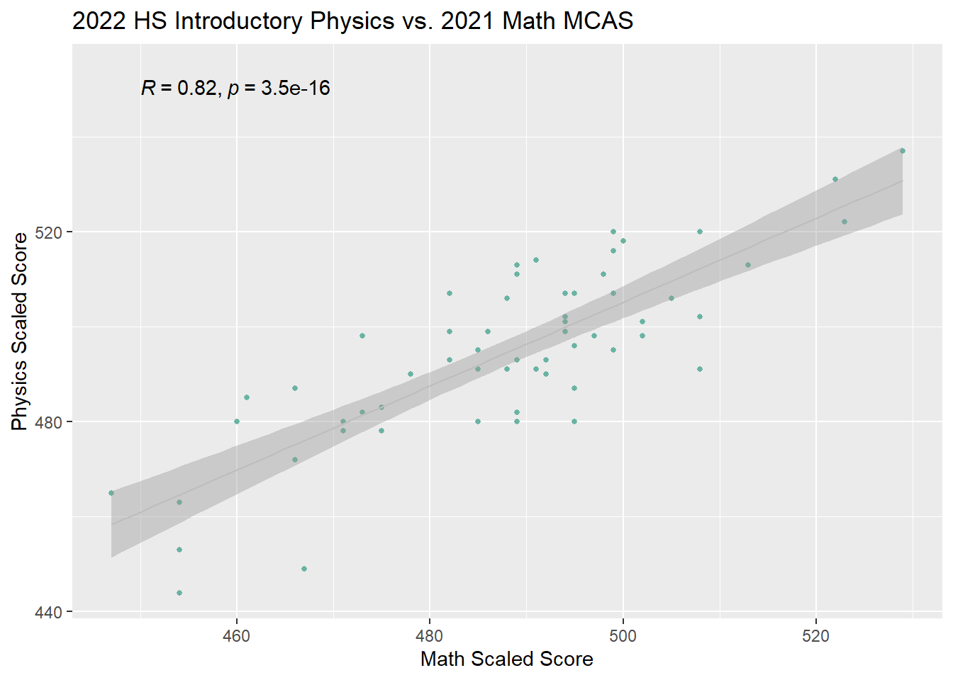
A student’s performance on their 9th Grade Introductory Physics MCAS is strongly associated with their performance on their 8th Grade Math MCAS exam. This suggests, we should use prior MCAS and current STAR Math testing data to identify students in need of extra support.
Code
G9Science_Math<-MCAS_2022%>%select(sscaleds, mscaleds2021,sscaleds_prior, grade, sattempt)%>%filter((grade ==9) & sattempt !="N")%>%ggplot(aes(x=`mscaleds2021`, y =`sscaleds`))+geom_point(size =1, color="#69b3a2")+geom_smooth(method="lm",color="grey", size =.5 )+labs(title ="2022 HS Introductory Physics vs. 2021 Math MCAS", y ="Physics Scaled Score",x ="Math Scaled Score") +stat_cor(method ="pearson", label.x =450, label.y =550)G9Science_Math
Rising Tide students performed slightly weaker relative to the state in all content reporting areas and lost the highest percentage of their points from items in Motion and Forces which is also represented in the most items on the exam.
Rising Tide students performed significantly weaker relative to students in the State on items including the key word Calculate in their item description. This suggests, we should dedicate more classroom instructional time to problem solving with calculation. Notably, the higher a student’s performance level, the higher the percentage of points a student lost for calculation items. To increase the proportion of students exceeding expectations, we need to improve our students performance on calculation based items; evidence based math interventions include small group, differentiated problem sets.
Students with disabilities performed better relative to their peers in the state while our non-disabled students performed worse. This further supports the need for differentiated small group problem sets in the general classroom setting.
Limitations/Areas for Improvement
To improve this report, I need to
edit down the number of visualizations used.
edit the average points lost by category to get average over all items, rather than average of averages.
mutate IEP so that the values 0 and 1 are Disabled and Non-Disabled
mutate Reporting Category so that the full category names appear in the graphs.
be more discerning on when to use totals and when to use averages. To improve performance on a test, we are concerned with total points lost; to identify curricular weaknesses we are also interested in relative performance to the state by content area
Here I would complete a key for all of the variables that are included in my table. And link relevant decoding documents from DESE
esgp, msgp, ssgpcontinuous: The student’s growth percentile. by subject area (e: English, m: Math, s: Science)
eperf2, mperf2, ordinal: The student’s performance level in ELA and Math
value
Key
Exceeds Expectations
E
Meets Expectations
M
Partially Meets Expectations
PM
Does Not Meet Expectations
NM
gender, nominal : the reported gender identify of the student.
value
Key
Female
F
Male
M
Non binary
N
Code
# examine the summary to decide how to best set up our data frameprint(summarytools::dfSummary(MCAS_2022,varnumbers =FALSE,plain.ascii =FALSE,style ="grid",graph.magnif =0.70,valid.col =FALSE),method ='render',table.classes ='table-condensed')
Data Frame Summary
MCAS_2022
Dimensions: 495 x 255
Duplicates: 0
Variable
Stats / Values
Freqs (% of Valid)
Graph
Missing
adminyear
[numeric]
1 distinct value
2022
:
495
(
100.0%
)
0
(0.0%)
testschoolcode
[character]
1. 4830305
495
(
100.0%
)
0
(0.0%)
grade
[factor]
1. 5
2. 6
3. 7
4. 8
5. 9
6. 10
89
(
18.0%
)
91
(
18.4%
)
92
(
18.6%
)
91
(
18.4%
)
69
(
13.9%
)
63
(
12.7%
)
0
(0.0%)
gradesims
[numeric]
Mean (sd) : 7.3 (1.6)
min ≤ med ≤ max:
5 ≤ 7 ≤ 10
IQR (CV) : 3 (0.2)
5
:
89
(
18.0%
)
6
:
91
(
18.4%
)
7
:
92
(
18.6%
)
8
:
91
(
18.4%
)
9
:
69
(
13.9%
)
10
:
63
(
12.7%
)
0
(0.0%)
dob
[Date]
min : 2005-02-08
med : 2008-11-29
max : 2011-10-17
range : 6y 8m 9d
427 distinct values
0
(0.0%)
gender
[character]
1. F
2. M
3. N
242
(
48.9%
)
251
(
50.7%
)
2
(
0.4%
)
0
(0.0%)
race
[character]
1. A
2. B
3. H
4. M
5. N
6. W
8
(
1.6%
)
6
(
1.2%
)
25
(
5.1%
)
41
(
8.3%
)
5
(
1.0%
)
410
(
82.8%
)
0
(0.0%)
yrsinmass
[character]
1. 1
2. 2
3. 3
4. 4
5. 5+
11
(
2.2%
)
18
(
3.6%
)
19
(
3.8%
)
16
(
3.2%
)
431
(
87.1%
)
0
(0.0%)
yrsinmass_num
[numeric]
Mean (sd) : 7.3 (2.4)
min ≤ med ≤ max:
1 ≤ 8 ≤ 12
IQR (CV) : 3 (0.3)
12 distinct values
0
(0.0%)
yrsinsch
[numeric]
Mean (sd) : 2.6 (1.5)
min ≤ med ≤ max:
1 ≤ 2 ≤ 6
IQR (CV) : 3 (0.6)
1
:
159
(
32.1%
)
2
:
116
(
23.4%
)
3
:
80
(
16.2%
)
4
:
77
(
15.6%
)
5
:
31
(
6.3%
)
6
:
32
(
6.5%
)
0
(0.0%)
highneeds
[character]
1. 0
2. 1
290
(
58.6%
)
205
(
41.4%
)
0
(0.0%)
lowincome
[character]
1. 0
2. 1
369
(
74.5%
)
126
(
25.5%
)
0
(0.0%)
title1
[character]
1. 0
2. 1
393
(
79.4%
)
102
(
20.6%
)
0
(0.0%)
ever_EL
[character]
1. 1
20
(
100.0%
)
475
(96.0%)
EL
[character]
1. 0
2. 1
488
(
98.6%
)
7
(
1.4%
)
0
(0.0%)
EL_FormerEL
[character]
1. 0
2. 1
480
(
97.0%
)
15
(
3.0%
)
0
(0.0%)
FormerEL
[character]
1. 0
2. 1
487
(
98.4%
)
8
(
1.6%
)
0
(0.0%)
ELfirstyear
[character]
All NA's
495
(100.0%)
IEP
[character]
1. 0
2. 1
381
(
77.0%
)
114
(
23.0%
)
0
(0.0%)
plan504
[character]
1. 0
2. 1
443
(
89.5%
)
52
(
10.5%
)
0
(0.0%)
firstlanguage
[character]
1. 2
2. 267
3. 415
4. 6
5. 630
6. 7
7. 759
1
(
0.2%
)
481
(
97.2%
)
2
(
0.4%
)
8
(
1.6%
)
1
(
0.2%
)
1
(
0.2%
)
1
(
0.2%
)
0
(0.0%)
natureofdis
[numeric]
Mean (sd) : 6.9 (1.9)
min ≤ med ≤ max:
2 ≤ 7 ≤ 12
IQR (CV) : 3 (0.3)
2
:
1
(
0.9%
)
3
:
9
(
7.8%
)
4
:
1
(
0.9%
)
5
:
19
(
16.5%
)
7
:
40
(
34.8%
)
8
:
38
(
33.0%
)
11
:
5
(
4.3%
)
12
:
2
(
1.7%
)
380
(76.8%)
levelofneed
[factor]
1. 1
2. 2
3. 3
4. 4
3
(
2.6%
)
14
(
12.2%
)
97
(
84.3%
)
1
(
0.9%
)
380
(76.8%)
spedplacement
[character]
1. 0
2. 1
3. 10
4. 20
380
(
76.8%
)
1
(
0.2%
)
104
(
21.0%
)
10
(
2.0%
)
0
(0.0%)
town
[character]
1. 239
2. 310
3. 52
4. 145
5. 182
6. 36
7. 20
8. 261
9. 171
10. 231
[ 11 others ]
257
(
51.9%
)
54
(
10.9%
)
33
(
6.7%
)
30
(
6.1%
)
23
(
4.6%
)
20
(
4.0%
)
18
(
3.6%
)
12
(
2.4%
)
11
(
2.2%
)
8
(
1.6%
)
29
(
5.9%
)
0
(0.0%)
county
[character]
1. Barnstable
2. Plymouth
56
(
11.3%
)
439
(
88.7%
)
0
(0.0%)
octenr
[numeric]
Min : 0
Mean : 1
Max : 1
0
:
13
(
2.6%
)
1
:
482
(
97.4%
)
0
(0.0%)
conenr_sch
[numeric]
1 distinct value
1
:
55
(
100.0%
)
440
(88.9%)
conenr_sta
[numeric]
1 distinct value
1
:
61
(
100.0%
)
434
(87.7%)
access_part
[numeric]
1 distinct value
1
:
7
(
100.0%
)
488
(98.6%)
ealt
[logical]
All NA's
495
(100.0%)
ecomplexity
[logical]
All NA's
495
(100.0%)
emode
[character]
1. O
422
(
100.0%
)
73
(14.7%)
eteststat
[character]
1. NTA
2. NTO
3. T
4
(
0.9%
)
1
(
0.2%
)
421
(
98.8%
)
69
(13.9%)
wptopdev
[logical]
All NA's
495
(100.0%)
wpcompconv
[logical]
All NA's
495
(100.0%)
eitem1
[numeric]
Min : 0
Mean : 0.8
Max : 1
0
:
95
(
22.6%
)
1
:
326
(
77.4%
)
74
(14.9%)
eitem2
[numeric]
Min : 0
Mean : 0.7
Max : 1
0
:
132
(
31.4%
)
1
:
289
(
68.6%
)
74
(14.9%)
eitem3
[numeric]
Min : 0
Mean : 0.8
Max : 1
0
:
91
(
21.6%
)
1
:
330
(
78.4%
)
74
(14.9%)
eitem4
[numeric]
Min : 0
Mean : 0.8
Max : 1
0
:
79
(
18.8%
)
1
:
342
(
81.2%
)
74
(14.9%)
eitem5
[numeric]
Mean (sd) : 0.9 (0.6)
min ≤ med ≤ max:
0 ≤ 1 ≤ 2
IQR (CV) : 1 (0.7)
0
:
109
(
25.9%
)
1
:
246
(
58.4%
)
2
:
66
(
15.7%
)
74
(14.9%)
eitem6
[numeric]
Min : 0
Mean : 0.8
Max : 1
0
:
97
(
23.0%
)
1
:
324
(
77.0%
)
74
(14.9%)
eitem7
[numeric]
Mean (sd) : 0.8 (0.5)
min ≤ med ≤ max:
0 ≤ 1 ≤ 2
IQR (CV) : 0 (0.6)
0
:
95
(
22.6%
)
1
:
307
(
72.9%
)
2
:
19
(
4.5%
)
74
(14.9%)
eitem8
[numeric]
Mean (sd) : 0.8 (0.5)
min ≤ med ≤ max:
0 ≤ 1 ≤ 2
IQR (CV) : 0 (0.6)
0
:
102
(
24.2%
)
1
:
292
(
69.4%
)
2
:
27
(
6.4%
)
74
(14.9%)
eitem9
[numeric]
Mean (sd) : 1.3 (1.5)
min ≤ med ≤ max:
0 ≤ 1 ≤ 7
IQR (CV) : 0 (1.2)
0
:
79
(
18.8%
)
1
:
285
(
67.7%
)
2
:
10
(
2.4%
)
4
:
20
(
4.8%
)
6
:
20
(
4.8%
)
7
:
7
(
1.7%
)
74
(14.9%)
eitem10
[numeric]
Mean (sd) : 1.2 (0.8)
min ≤ med ≤ max:
0 ≤ 1 ≤ 2
IQR (CV) : 2 (0.7)
0
:
107
(
25.4%
)
1
:
124
(
29.5%
)
2
:
190
(
45.1%
)
74
(14.9%)
eitem11
[numeric]
Mean (sd) : 1.2 (0.7)
min ≤ med ≤ max:
0 ≤ 1 ≤ 2
IQR (CV) : 1 (0.5)
0
:
54
(
12.8%
)
1
:
208
(
49.4%
)
2
:
159
(
37.8%
)
74
(14.9%)
eitem12
[numeric]
Mean (sd) : 2.5 (2.3)
min ≤ med ≤ max:
0 ≤ 1 ≤ 8
IQR (CV) : 3 (0.9)
0
:
69
(
16.4%
)
1
:
152
(
36.1%
)
2
:
33
(
7.8%
)
3
:
6
(
1.4%
)
4
:
80
(
19.0%
)
5
:
7
(
1.7%
)
6
:
50
(
11.9%
)
7
:
18
(
4.3%
)
8
:
6
(
1.4%
)
74
(14.9%)
eitem13
[numeric]
Mean (sd) : 1.4 (1.5)
min ≤ med ≤ max:
0 ≤ 1 ≤ 7
IQR (CV) : 1 (1)
0
:
88
(
21.0%
)
1
:
218
(
51.9%
)
2
:
56
(
13.3%
)
3
:
8
(
1.9%
)
4
:
27
(
6.4%
)
5
:
3
(
0.7%
)
6
:
18
(
4.3%
)
7
:
2
(
0.5%
)
75
(15.2%)
eitem14
[numeric]
Min : 0
Mean : 0.8
Max : 1
0
:
104
(
24.6%
)
1
:
318
(
75.4%
)
73
(14.7%)
eitem15
[numeric]
Mean (sd) : 0.9 (0.6)
min ≤ med ≤ max:
0 ≤ 1 ≤ 2
IQR (CV) : 0 (0.7)
0
:
101
(
23.9%
)
1
:
260
(
61.6%
)
2
:
61
(
14.5%
)
73
(14.7%)
eitem16
[numeric]
Min : 0
Mean : 0.8
Max : 1
0
:
76
(
18.0%
)
1
:
346
(
82.0%
)
73
(14.7%)
eitem17
[numeric]
Min : 0
Mean : 0.7
Max : 1
0
:
122
(
28.9%
)
1
:
300
(
71.1%
)
73
(14.7%)
eitem18
[numeric]
Min : 0
Mean : 0.7
Max : 1
0
:
110
(
26.1%
)
1
:
312
(
73.9%
)
73
(14.7%)
eitem19
[numeric]
Mean (sd) : 0.9 (0.7)
min ≤ med ≤ max:
0 ≤ 1 ≤ 2
IQR (CV) : 1 (0.7)
0
:
110
(
26.1%
)
1
:
234
(
55.5%
)
2
:
78
(
18.5%
)
73
(14.7%)
eitem20
[numeric]
Mean (sd) : 1 (0.6)
min ≤ med ≤ max:
0 ≤ 1 ≤ 2
IQR (CV) : 0 (0.6)
0
:
61
(
14.5%
)
1
:
281
(
66.6%
)
2
:
80
(
19.0%
)
73
(14.7%)
eitem21
[numeric]
Mean (sd) : 1 (0.5)
min ≤ med ≤ max:
0 ≤ 1 ≤ 2
IQR (CV) : 0 (0.5)
0
:
64
(
15.2%
)
1
:
309
(
73.2%
)
2
:
49
(
11.6%
)
73
(14.7%)
eitem22
[numeric]
Mean (sd) : 1.4 (1.5)
min ≤ med ≤ max:
0 ≤ 1 ≤ 7
IQR (CV) : 0 (1.1)
0
:
51
(
12.1%
)
1
:
310
(
73.5%
)
2
:
10
(
2.4%
)
4
:
23
(
5.5%
)
6
:
19
(
4.5%
)
7
:
9
(
2.1%
)
73
(14.7%)
eitem23
[numeric]
Mean (sd) : 0.8 (0.6)
min ≤ med ≤ max:
0 ≤ 1 ≤ 2
IQR (CV) : 1 (0.7)
0
:
124
(
29.4%
)
1
:
252
(
59.7%
)
2
:
46
(
10.9%
)
73
(14.7%)
eitem24
[numeric]
Mean (sd) : 0.9 (0.6)
min ≤ med ≤ max:
0 ≤ 1 ≤ 2
IQR (CV) : 0 (0.6)
0
:
81
(
19.2%
)
1
:
287
(
68.0%
)
2
:
54
(
12.8%
)
73
(14.7%)
eitem25
[numeric]
Mean (sd) : 0.9 (0.6)
min ≤ med ≤ max:
0 ≤ 1 ≤ 2
IQR (CV) : 0 (0.6)
0
:
84
(
19.9%
)
1
:
285
(
67.5%
)
2
:
53
(
12.6%
)
73
(14.7%)
eitem26
[numeric]
Min : 0
Mean : 0.7
Max : 1
0
:
121
(
28.7%
)
1
:
301
(
71.3%
)
73
(14.7%)
eitem27
[numeric]
Mean (sd) : 0.9 (0.6)
min ≤ med ≤ max:
0 ≤ 1 ≤ 2
IQR (CV) : 0 (0.6)
0
:
89
(
21.1%
)
1
:
272
(
64.5%
)
2
:
61
(
14.5%
)
73
(14.7%)
eitem28
[numeric]
Mean (sd) : 0.9 (0.6)
min ≤ med ≤ max:
0 ≤ 1 ≤ 2
IQR (CV) : 0 (0.6)
0
:
86
(
20.4%
)
1
:
283
(
67.1%
)
2
:
53
(
12.6%
)
73
(14.7%)
eitem29
[numeric]
Mean (sd) : 0.8 (0.6)
min ≤ med ≤ max:
0 ≤ 1 ≤ 2
IQR (CV) : 1 (0.7)
0
:
123
(
29.1%
)
1
:
256
(
60.7%
)
2
:
43
(
10.2%
)
73
(14.7%)
eitem30
[numeric]
Mean (sd) : 1.2 (0.7)
min ≤ med ≤ max:
0 ≤ 1 ≤ 2
IQR (CV) : 1 (0.6)
0
:
67
(
15.9%
)
1
:
219
(
51.9%
)
2
:
136
(
32.2%
)
73
(14.7%)
eitem31
[numeric]
Mean (sd) : 3.2 (2.2)
min ≤ med ≤ max:
0 ≤ 3 ≤ 8
IQR (CV) : 4 (0.7)
0
:
25
(
6.9%
)
1
:
70
(
19.4%
)
2
:
81
(
22.5%
)
3
:
21
(
5.8%
)
4
:
69
(
19.2%
)
5
:
14
(
3.9%
)
6
:
55
(
15.3%
)
7
:
17
(
4.7%
)
8
:
8
(
2.2%
)
135
(27.3%)
eitem32
[numeric]
Mean (sd) : 3.2 (1.7)
min ≤ med ≤ max:
0 ≤ 3.5 ≤ 8
IQR (CV) : 2 (0.5)
0
:
5
(
5.4%
)
1
:
5
(
5.4%
)
2
:
32
(
34.8%
)
3
:
4
(
4.3%
)
4
:
34
(
37.0%
)
5
:
1
(
1.1%
)
6
:
10
(
10.9%
)
8
:
1
(
1.1%
)
403
(81.4%)
eitem33
[logical]
All NA's
495
(100.0%)
eitem34
[logical]
All NA's
495
(100.0%)
eitem35
[logical]
All NA's
495
(100.0%)
eitem36
[logical]
All NA's
495
(100.0%)
eitem37
[logical]
All NA's
495
(100.0%)
eitem38
[logical]
All NA's
495
(100.0%)
eitem39
[logical]
All NA's
495
(100.0%)
eitem40
[logical]
All NA's
495
(100.0%)
erawsc
[numeric]
Mean (sd) : 33 (8.2)
min ≤ med ≤ max:
6 ≤ 34 ≤ 47
IQR (CV) : 10 (0.2)
39 distinct values
73
(14.7%)
emcpts
[numeric]
Mean (sd) : 18.3 (4.1)
min ≤ med ≤ max:
3 ≤ 19 ≤ 26
IQR (CV) : 5 (0.2)
24 distinct values
73
(14.7%)
eorpts
[numeric]
Mean (sd) : 14.7 (5.4)
min ≤ med ≤ max:
1 ≤ 15 ≤ 28
IQR (CV) : 8 (0.4)
28 distinct values
73
(14.7%)
eperpospts
[numeric]
Mean (sd) : 66.3 (16.3)
min ≤ med ≤ max:
12 ≤ 69 ≤ 94
IQR (CV) : 20 (0.2)
63 distinct values
73
(14.7%)
escaleds
[numeric]
Mean (sd) : 501.3 (18.5)
min ≤ med ≤ max:
442 ≤ 502 ≤ 545
IQR (CV) : 25 (0)
74 distinct values
74
(14.9%)
eperflev
[ordered, factor]
1. E
2. M
3. PM
4. NM
5. DNT
6. ABS
24
(
5.6%
)
206
(
48.4%
)
169
(
39.7%
)
22
(
5.2%
)
1
(
0.2%
)
4
(
0.9%
)
69
(13.9%)
eperf2
[ordered, factor]
1. E
2. M
3. PM
4. NM
24
(
5.7%
)
206
(
48.9%
)
169
(
40.1%
)
22
(
5.2%
)
74
(14.9%)
enumin
[numeric]
1 distinct value
1
:
421
(
100.0%
)
74
(14.9%)
eassess
[numeric]
Min : 0
Mean : 1
Max : 1
0
:
4
(
0.9%
)
1
:
421
(
99.1%
)
70
(14.1%)
esgp
[numeric]
Mean (sd) : 52.6 (29.6)
min ≤ med ≤ max:
1 ≤ 54 ≤ 99
IQR (CV) : 48.5 (0.6)
96 distinct values
109
(22.0%)
idea1
[character]
1. 0
2. 1
3. 2
4. 3
5. 4
6. 5
7. BL
8. OT
70
(
16.4%
)
79
(
18.5%
)
138
(
32.4%
)
97
(
22.8%
)
27
(
6.3%
)
6
(
1.4%
)
7
(
1.6%
)
2
(
0.5%
)
69
(13.9%)
conv1
[character]
1. 0
2. 1
3. 2
4. 3
5. BL
6. OT
34
(
8.0%
)
121
(
28.4%
)
140
(
32.9%
)
122
(
28.6%
)
7
(
1.6%
)
2
(
0.5%
)
69
(13.9%)
idea2
[character]
1. 0
2. 1
3. 2
4. 3
5. 4
6. 5
7. BL
8. OT
21
(
4.9%
)
121
(
28.4%
)
146
(
34.3%
)
96
(
22.5%
)
27
(
6.3%
)
9
(
2.1%
)
4
(
0.9%
)
2
(
0.5%
)
69
(13.9%)
conv2
[character]
1. 0
2. 1
3. 2
4. 3
5. BL
6. OT
33
(
7.7%
)
121
(
28.4%
)
145
(
34.0%
)
121
(
28.4%
)
4
(
0.9%
)
2
(
0.5%
)
69
(13.9%)
idea3
[logical]
All NA's
495
(100.0%)
conv3
[logical]
All NA's
495
(100.0%)
eattempt
[character]
1. F
2. N
3. P
421
(
98.8%
)
4
(
0.9%
)
1
(
0.2%
)
69
(13.9%)
malt
[logical]
All NA's
495
(100.0%)
mcomplexity
[logical]
All NA's
495
(100.0%)
mmode
[character]
1. O
424
(
100.0%
)
71
(14.3%)
mteststat
[character]
1. NTA
2. NTO
3. T
2
(
0.5%
)
1
(
0.2%
)
423
(
99.3%
)
69
(13.9%)
mitem1
[numeric]
Min : 0
Mean : 0.8
Max : 1
0
:
94
(
22.3%
)
1
:
328
(
77.7%
)
73
(14.7%)
mitem2
[numeric]
Min : 0
Mean : 0.7
Max : 1
0
:
127
(
30.1%
)
1
:
295
(
69.9%
)
73
(14.7%)
mitem3
[numeric]
Min : 0
Mean : 0.6
Max : 1
0
:
174
(
41.2%
)
1
:
248
(
58.8%
)
73
(14.7%)
mitem4
[numeric]
Mean (sd) : 1.1 (1.1)
min ≤ med ≤ max:
0 ≤ 1 ≤ 4
IQR (CV) : 2 (1)
0
:
156
(
37.1%
)
1
:
148
(
35.2%
)
2
:
55
(
13.1%
)
3
:
42
(
10.0%
)
4
:
19
(
4.5%
)
75
(15.2%)
mitem5
[numeric]
Min : 0
Mean : 0.4
Max : 1
0
:
237
(
56.3%
)
1
:
184
(
43.7%
)
74
(14.9%)
mitem6
[numeric]
Mean (sd) : 0.9 (0.9)
min ≤ med ≤ max:
0 ≤ 1 ≤ 4
IQR (CV) : 1 (1)
0
:
151
(
35.8%
)
1
:
219
(
51.9%
)
2
:
19
(
4.5%
)
3
:
22
(
5.2%
)
4
:
11
(
2.6%
)
73
(14.7%)
mitem7
[numeric]
Mean (sd) : 0.6 (0.7)
min ≤ med ≤ max:
0 ≤ 0 ≤ 2
IQR (CV) : 1 (1.1)
0
:
213
(
50.5%
)
1
:
159
(
37.7%
)
2
:
50
(
11.8%
)
73
(14.7%)
mitem8
[numeric]
Mean (sd) : 0.8 (0.9)
min ≤ med ≤ max:
0 ≤ 1 ≤ 4
IQR (CV) : 1 (1.1)
0
:
182
(
43.4%
)
1
:
167
(
39.9%
)
2
:
54
(
12.9%
)
3
:
7
(
1.7%
)
4
:
9
(
2.1%
)
76
(15.4%)
mitem9
[numeric]
Mean (sd) : 0.8 (0.9)
min ≤ med ≤ max:
0 ≤ 1 ≤ 4
IQR (CV) : 1 (1)
0
:
150
(
35.5%
)
1
:
225
(
53.3%
)
2
:
27
(
6.4%
)
3
:
8
(
1.9%
)
4
:
12
(
2.8%
)
73
(14.7%)
mitem10
[numeric]
Min : 0
Mean : 0.6
Max : 1
0
:
183
(
43.4%
)
1
:
239
(
56.6%
)
73
(14.7%)
mitem11
[numeric]
Mean (sd) : 0.7 (0.5)
min ≤ med ≤ max:
0 ≤ 1 ≤ 2
IQR (CV) : 1 (0.7)
0
:
123
(
29.1%
)
1
:
288
(
68.2%
)
2
:
11
(
2.6%
)
73
(14.7%)
mitem12
[numeric]
Mean (sd) : 0.8 (0.8)
min ≤ med ≤ max:
0 ≤ 1 ≤ 4
IQR (CV) : 1 (1)
0
:
161
(
38.2%
)
1
:
222
(
52.6%
)
2
:
23
(
5.5%
)
3
:
9
(
2.1%
)
4
:
7
(
1.7%
)
73
(14.7%)
mitem13
[numeric]
Mean (sd) : 1.2 (1.3)
min ≤ med ≤ max:
0 ≤ 1 ≤ 4
IQR (CV) : 1 (1.1)
0
:
156
(
37.0%
)
1
:
164
(
38.9%
)
2
:
24
(
5.7%
)
3
:
34
(
8.1%
)
4
:
44
(
10.4%
)
73
(14.7%)
mitem14
[numeric]
Mean (sd) : 1.1 (1)
min ≤ med ≤ max:
0 ≤ 1 ≤ 4
IQR (CV) : 0 (0.9)
0
:
102
(
24.2%
)
1
:
229
(
54.3%
)
2
:
47
(
11.1%
)
3
:
16
(
3.8%
)
4
:
28
(
6.6%
)
73
(14.7%)
mitem15
[numeric]
Mean (sd) : 0.5 (0.6)
min ≤ med ≤ max:
0 ≤ 0 ≤ 3
IQR (CV) : 1 (1.3)
0
:
242
(
57.8%
)
1
:
153
(
36.5%
)
2
:
20
(
4.8%
)
3
:
4
(
1.0%
)
76
(15.4%)
mitem16
[numeric]
Min : 0
Mean : 0.5
Max : 1
0
:
223
(
53.0%
)
1
:
198
(
47.0%
)
74
(14.9%)
mitem17
[numeric]
Mean (sd) : 0.5 (0.6)
min ≤ med ≤ max:
0 ≤ 0 ≤ 2
IQR (CV) : 1 (1.1)
0
:
219
(
52.0%
)
1
:
187
(
44.4%
)
2
:
15
(
3.6%
)
74
(14.9%)
mitem18
[numeric]
Mean (sd) : 0.5 (0.6)
min ≤ med ≤ max:
0 ≤ 0 ≤ 2
IQR (CV) : 1 (1.1)
0
:
221
(
52.4%
)
1
:
186
(
44.1%
)
2
:
15
(
3.6%
)
73
(14.7%)
mitem19
[numeric]
Min : 0
Mean : 0.3
Max : 1
0
:
285
(
67.7%
)
1
:
136
(
32.3%
)
74
(14.9%)
mitem20
[numeric]
Min : 0
Mean : 0.4
Max : 1
0
:
242
(
57.3%
)
1
:
180
(
42.7%
)
73
(14.7%)
mitem21
[numeric]
Min : 0
Mean : 0.8
Max : 1
0
:
82
(
19.4%
)
1
:
340
(
80.6%
)
73
(14.7%)
mitem22
[numeric]
Mean (sd) : 1 (0.8)
min ≤ med ≤ max:
0 ≤ 1 ≤ 4
IQR (CV) : 0 (0.8)
0
:
81
(
19.2%
)
1
:
291
(
69.1%
)
2
:
19
(
4.5%
)
3
:
20
(
4.8%
)
4
:
10
(
2.4%
)
74
(14.9%)
mitem23
[numeric]
Mean (sd) : 0.8 (0.9)
min ≤ med ≤ max:
0 ≤ 1 ≤ 4
IQR (CV) : 1 (1.1)
0
:
157
(
37.2%
)
1
:
223
(
52.8%
)
2
:
16
(
3.8%
)
3
:
6
(
1.4%
)
4
:
20
(
4.7%
)
73
(14.7%)
mitem24
[numeric]
Mean (sd) : 0.9 (0.9)
min ≤ med ≤ max:
0 ≤ 1 ≤ 4
IQR (CV) : 1 (1.1)
0
:
165
(
39.1%
)
1
:
187
(
44.3%
)
2
:
46
(
10.9%
)
3
:
12
(
2.8%
)
4
:
12
(
2.8%
)
73
(14.7%)
mitem25
[numeric]
Min : 0
Mean : 0.6
Max : 1
0
:
179
(
42.6%
)
1
:
241
(
57.4%
)
75
(15.2%)
mitem26
[numeric]
Mean (sd) : 1 (1)
min ≤ med ≤ max:
0 ≤ 1 ≤ 4
IQR (CV) : 1 (1)
0
:
158
(
37.4%
)
1
:
172
(
40.7%
)
2
:
58
(
13.7%
)
3
:
24
(
5.7%
)
4
:
11
(
2.6%
)
72
(14.5%)
mitem27
[numeric]
Mean (sd) : 0.8 (1)
min ≤ med ≤ max:
0 ≤ 1 ≤ 4
IQR (CV) : 1 (1.3)
0
:
194
(
46.1%
)
1
:
181
(
43.0%
)
2
:
16
(
3.8%
)
3
:
14
(
3.3%
)
4
:
16
(
3.8%
)
74
(14.9%)
mitem28
[numeric]
Mean (sd) : 0.7 (0.7)
min ≤ med ≤ max:
0 ≤ 1 ≤ 2
IQR (CV) : 1 (1)
0
:
182
(
43.2%
)
1
:
190
(
45.1%
)
2
:
49
(
11.6%
)
74
(14.9%)
mitem29
[numeric]
Min : 0
Mean : 0.5
Max : 1
0
:
208
(
49.4%
)
1
:
213
(
50.6%
)
74
(14.9%)
mitem30
[numeric]
Mean (sd) : 0.6 (0.6)
min ≤ med ≤ max:
0 ≤ 1 ≤ 2
IQR (CV) : 1 (1)
0
:
192
(
45.5%
)
1
:
195
(
46.2%
)
2
:
35
(
8.3%
)
73
(14.7%)
mitem31
[numeric]
Mean (sd) : 0.9 (0.9)
min ≤ med ≤ max:
0 ≤ 1 ≤ 4
IQR (CV) : 1 (1)
0
:
133
(
31.6%
)
1
:
241
(
57.2%
)
2
:
19
(
4.5%
)
3
:
17
(
4.0%
)
4
:
11
(
2.6%
)
74
(14.9%)
mitem32
[numeric]
Mean (sd) : 0.5 (0.6)
min ≤ med ≤ max:
0 ≤ 0 ≤ 2
IQR (CV) : 1 (1.2)
0
:
240
(
56.9%
)
1
:
170
(
40.3%
)
2
:
12
(
2.8%
)
73
(14.7%)
mitem33
[numeric]
Min : 0
Mean : 0.5
Max : 1
0
:
216
(
51.2%
)
1
:
206
(
48.8%
)
73
(14.7%)
mitem34
[numeric]
Mean (sd) : 0.7 (0.8)
min ≤ med ≤ max:
0 ≤ 1 ≤ 4
IQR (CV) : 1 (1.2)
0
:
190
(
45.1%
)
1
:
191
(
45.4%
)
2
:
20
(
4.8%
)
3
:
15
(
3.6%
)
4
:
5
(
1.2%
)
74
(14.9%)
mitem35
[numeric]
Mean (sd) : 0.8 (0.8)
min ≤ med ≤ max:
0 ≤ 1 ≤ 4
IQR (CV) : 1 (1.1)
0
:
168
(
39.8%
)
1
:
200
(
47.4%
)
2
:
33
(
7.8%
)
3
:
15
(
3.6%
)
4
:
6
(
1.4%
)
73
(14.7%)
mitem36
[numeric]
Min : 0
Mean : 0.4
Max : 1
0
:
238
(
56.5%
)
1
:
183
(
43.5%
)
74
(14.9%)
mitem37
[numeric]
Mean (sd) : 1.1 (1.2)
min ≤ med ≤ max:
0 ≤ 1 ≤ 4
IQR (CV) : 1 (1.1)
0
:
153
(
36.3%
)
1
:
187
(
44.3%
)
2
:
13
(
3.1%
)
3
:
36
(
8.5%
)
4
:
33
(
7.8%
)
73
(14.7%)
mitem38
[numeric]
Min : 0
Mean : 0.5
Max : 1
0
:
216
(
51.3%
)
1
:
205
(
48.7%
)
74
(14.9%)
mitem39
[numeric]
Mean (sd) : 0.3 (0.6)
min ≤ med ≤ max:
0 ≤ 0 ≤ 2
IQR (CV) : 1 (1.6)
0
:
296
(
70.1%
)
1
:
106
(
25.1%
)
2
:
20
(
4.7%
)
73
(14.7%)
mitem40
[numeric]
Min : 0
Mean : 0.5
Max : 1
0
:
221
(
52.4%
)
1
:
201
(
47.6%
)
73
(14.7%)
mitem41
[numeric]
Min : 0
Mean : 0.5
Max : 1
0
:
31
(
49.2%
)
1
:
32
(
50.8%
)
432
(87.3%)
mitem42
[numeric]
Min : 0
Mean : 0.5
Max : 1
0
:
31
(
49.2%
)
1
:
32
(
50.8%
)
432
(87.3%)
mrawsc
[numeric]
Mean (sd) : 27.6 (11.2)
min ≤ med ≤ max:
0 ≤ 27 ≤ 58
IQR (CV) : 15 (0.4)
51 distinct values
72
(14.5%)
mmcpts
[numeric]
Mean (sd) : 10.5 (4)
min ≤ med ≤ max:
0 ≤ 10 ≤ 21
IQR (CV) : 5 (0.4)
22 distinct values
72
(14.5%)
morpts
[numeric]
Mean (sd) : 17.2 (8.1)
min ≤ med ≤ max:
0 ≤ 16 ≤ 38
IQR (CV) : 12 (0.5)
38 distinct values
72
(14.5%)
mperpospts
[numeric]
Mean (sd) : 50.3 (20.3)
min ≤ med ≤ max:
0 ≤ 50 ≤ 97
IQR (CV) : 28 (0.4)
67 distinct values
72
(14.5%)
mscaleds
[numeric]
Mean (sd) : 497.3 (17.6)
min ≤ med ≤ max:
440 ≤ 498 ≤ 555
IQR (CV) : 20 (0)
80 distinct values
72
(14.5%)
mperflev
[ordered, factor]
1. E
2. M
3. PM
4. NM
5. INV
6. ABS
13
(
3.1%
)
168
(
39.4%
)
209
(
49.1%
)
33
(
7.7%
)
1
(
0.2%
)
2
(
0.5%
)
69
(13.9%)
mperf2
[ordered, factor]
1. E
2. M
3. PM
4. NM
13
(
3.1%
)
168
(
39.7%
)
209
(
49.4%
)
33
(
7.8%
)
72
(14.5%)
mnumin
[numeric]
1 distinct value
1
:
423
(
100.0%
)
72
(14.5%)
massess
[numeric]
Min : 0
Mean : 1
Max : 1
0
:
2
(
0.5%
)
1
:
423
(
99.5%
)
70
(14.1%)
msgp
[numeric]
Mean (sd) : 43.7 (27.6)
min ≤ med ≤ max:
1 ≤ 40 ≤ 99
IQR (CV) : 46 (0.6)
97 distinct values
107
(21.6%)
mattempt
[character]
1. F
2. N
424
(
99.5%
)
2
(
0.5%
)
69
(13.9%)
salt
[logical]
All NA's
495
(100.0%)
scomplexity
[logical]
All NA's
495
(100.0%)
smode
[character]
1. O
2. P
248
(
96.9%
)
8
(
3.1%
)
239
(48.3%)
steststat
[character]
1. NTA
2. NTO
3. T
4. TR
2
(
0.6%
)
54
(
17.3%
)
250
(
80.1%
)
6
(
1.9%
)
183
(37.0%)
ssubject
[character]
1. 1
2. 2
3. 3
4. 6
3
(
2.3%
)
8
(
6.1%
)
51
(
38.6%
)
70
(
53.0%
)
363
(73.3%)
sitem1
[numeric]
Min : 0
Mean : 0.9
Max : 1
0
:
36
(
14.1%
)
1
:
220
(
85.9%
)
239
(48.3%)
sitem2
[numeric]
Min : 0
Mean : 0.6
Max : 1
0
:
109
(
42.6%
)
1
:
147
(
57.4%
)
239
(48.3%)
sitem3
[numeric]
Min : 0
Mean : 0.6
Max : 1
0
:
110
(
43.0%
)
1
:
146
(
57.0%
)
239
(48.3%)
sitem4
[numeric]
Min : 0
Mean : 0.6
Max : 1
0
:
102
(
40.0%
)
1
:
153
(
60.0%
)
240
(48.5%)
sitem5
[numeric]
Mean (sd) : 1 (0.7)
min ≤ med ≤ max:
0 ≤ 1 ≤ 2
IQR (CV) : 2 (0.7)
0
:
66
(
25.8%
)
1
:
125
(
48.8%
)
2
:
65
(
25.4%
)
239
(48.3%)
sitem6
[numeric]
Mean (sd) : 0.9 (0.7)
min ≤ med ≤ max:
0 ≤ 1 ≤ 2
IQR (CV) : 1 (0.8)
0
:
77
(
30.1%
)
1
:
119
(
46.5%
)
2
:
60
(
23.4%
)
239
(48.3%)
sitem7
[numeric]
Min : 0
Mean : 0.6
Max : 1
0
:
113
(
44.1%
)
1
:
143
(
55.9%
)
239
(48.3%)
sitem8
[numeric]
Min : 0
Mean : 0.5
Max : 1
0
:
131
(
51.2%
)
1
:
125
(
48.8%
)
239
(48.3%)
sitem9
[numeric]
Min : 0
Mean : 0.7
Max : 1
0
:
65
(
25.4%
)
1
:
191
(
74.6%
)
239
(48.3%)
sitem10
[numeric]
Min : 0
Mean : 0.7
Max : 1
0
:
85
(
33.2%
)
1
:
171
(
66.8%
)
239
(48.3%)
sitem11
[numeric]
Mean (sd) : 0.6 (0.6)
min ≤ med ≤ max:
0 ≤ 1 ≤ 4
IQR (CV) : 1 (1)
0
:
113
(
44.1%
)
1
:
139
(
54.3%
)
2
:
2
(
0.8%
)
3
:
1
(
0.4%
)
4
:
1
(
0.4%
)
239
(48.3%)
sitem12
[numeric]
Min : 0
Mean : 0.6
Max : 1
0
:
102
(
40.0%
)
1
:
153
(
60.0%
)
240
(48.5%)
sitem13
[numeric]
Mean (sd) : 0.9 (0.5)
min ≤ med ≤ max:
0 ≤ 1 ≤ 2
IQR (CV) : 0 (0.6)
0
:
42
(
16.4%
)
1
:
186
(
72.7%
)
2
:
28
(
10.9%
)
239
(48.3%)
sitem14
[numeric]
Min : 0
Mean : 0.6
Max : 1
0
:
101
(
39.5%
)
1
:
155
(
60.5%
)
239
(48.3%)
sitem15
[numeric]
Mean (sd) : 1.4 (0.9)
min ≤ med ≤ max:
0 ≤ 1 ≤ 3
IQR (CV) : 1 (0.6)
0
:
45
(
17.6%
)
1
:
86
(
33.6%
)
2
:
100
(
39.1%
)
3
:
25
(
9.8%
)
239
(48.3%)
sitem16
[numeric]
Mean (sd) : 1.1 (0.8)
min ≤ med ≤ max:
0 ≤ 1 ≤ 3
IQR (CV) : 2 (0.7)
0
:
65
(
25.7%
)
1
:
110
(
43.5%
)
2
:
72
(
28.5%
)
3
:
6
(
2.4%
)
242
(48.9%)
sitem17
[numeric]
Mean (sd) : 1 (0.8)
min ≤ med ≤ max:
0 ≤ 1 ≤ 3
IQR (CV) : 1 (0.8)
0
:
68
(
26.7%
)
1
:
126
(
49.4%
)
2
:
49
(
19.2%
)
3
:
12
(
4.7%
)
240
(48.5%)
sitem18
[numeric]
Mean (sd) : 0.9 (0.7)
min ≤ med ≤ max:
0 ≤ 1 ≤ 2
IQR (CV) : 1 (0.7)
0
:
70
(
27.3%
)
1
:
133
(
52.0%
)
2
:
53
(
20.7%
)
239
(48.3%)
sitem19
[numeric]
Min : 0
Mean : 0.6
Max : 1
0
:
110
(
43.0%
)
1
:
146
(
57.0%
)
239
(48.3%)
sitem20
[numeric]
Mean (sd) : 1 (0.9)
min ≤ med ≤ max:
0 ≤ 1 ≤ 4
IQR (CV) : 1 (0.9)
0
:
78
(
30.6%
)
1
:
132
(
51.8%
)
2
:
24
(
9.4%
)
3
:
17
(
6.7%
)
4
:
4
(
1.6%
)
240
(48.5%)
sitem21
[numeric]
Mean (sd) : 0.8 (0.6)
min ≤ med ≤ max:
0 ≤ 1 ≤ 3
IQR (CV) : 0 (0.7)
0
:
62
(
24.6%
)
1
:
175
(
69.4%
)
2
:
11
(
4.4%
)
3
:
4
(
1.6%
)
243
(49.1%)
sitem22
[numeric]
Min : 0
Mean : 0.7
Max : 1
0
:
76
(
29.7%
)
1
:
180
(
70.3%
)
239
(48.3%)
sitem23
[numeric]
Min : 0
Mean : 0.6
Max : 1
0
:
95
(
37.3%
)
1
:
160
(
62.7%
)
240
(48.5%)
sitem24
[numeric]
Min : 0
Mean : 0.7
Max : 1
0
:
73
(
28.5%
)
1
:
183
(
71.5%
)
239
(48.3%)
sitem25
[numeric]
Mean (sd) : 0.7 (0.6)
min ≤ med ≤ max:
0 ≤ 1 ≤ 2
IQR (CV) : 1 (0.9)
0
:
105
(
41.0%
)
1
:
127
(
49.6%
)
2
:
24
(
9.4%
)
239
(48.3%)
sitem26
[numeric]
Min : 0
Mean : 0.6
Max : 1
0
:
104
(
40.6%
)
1
:
152
(
59.4%
)
239
(48.3%)
sitem27
[numeric]
Mean (sd) : 1.5 (0.8)
min ≤ med ≤ max:
0 ≤ 1 ≤ 3
IQR (CV) : 1 (0.6)
0
:
24
(
9.4%
)
1
:
112
(
43.8%
)
2
:
90
(
35.2%
)
3
:
30
(
11.7%
)
239
(48.3%)
sitem28
[numeric]
Mean (sd) : 1.2 (1)
min ≤ med ≤ max:
0 ≤ 1 ≤ 3
IQR (CV) : 2 (0.9)
0
:
78
(
30.6%
)
1
:
83
(
32.5%
)
2
:
61
(
23.9%
)
3
:
33
(
12.9%
)
240
(48.5%)
sitem29
[numeric]
Mean (sd) : 1 (0.7)
min ≤ med ≤ max:
0 ≤ 1 ≤ 2
IQR (CV) : 1.2 (0.7)
0
:
64
(
25.0%
)
1
:
124
(
48.4%
)
2
:
68
(
26.6%
)
239
(48.3%)
sitem30
[numeric]
Mean (sd) : 0.6 (0.5)
min ≤ med ≤ max:
0 ≤ 1 ≤ 2
IQR (CV) : 1 (0.9)
0
:
108
(
42.2%
)
1
:
147
(
57.4%
)
2
:
1
(
0.4%
)
239
(48.3%)
sitem31
[numeric]
Min : 0
Mean : 0.6
Max : 1
0
:
95
(
37.1%
)
1
:
161
(
62.9%
)
239
(48.3%)
sitem32
[numeric]
Min : 0
Mean : 0.7
Max : 1
0
:
88
(
34.4%
)
1
:
168
(
65.6%
)
239
(48.3%)
sitem33
[numeric]
Mean (sd) : 0.8 (0.4)
min ≤ med ≤ max:
0 ≤ 1 ≤ 2
IQR (CV) : 0 (0.6)
0
:
58
(
22.7%
)
1
:
194
(
76.1%
)
2
:
3
(
1.2%
)
240
(48.5%)
sitem34
[numeric]
Min : 0
Mean : 0.5
Max : 1
0
:
137
(
53.5%
)
1
:
119
(
46.5%
)
239
(48.3%)
sitem35
[numeric]
Min : 0
Mean : 0.4
Max : 1
0
:
141
(
55.1%
)
1
:
115
(
44.9%
)
239
(48.3%)
sitem36
[numeric]
Mean (sd) : 0.9 (0.7)
min ≤ med ≤ max:
0 ≤ 1 ≤ 2
IQR (CV) : 1 (0.8)
0
:
75
(
29.4%
)
1
:
135
(
52.9%
)
2
:
45
(
17.6%
)
240
(48.5%)
sitem37
[numeric]
Mean (sd) : 0.7 (0.8)
min ≤ med ≤ max:
0 ≤ 1 ≤ 3
IQR (CV) : 1 (1.1)
0
:
112
(
43.8%
)
1
:
109
(
42.6%
)
2
:
26
(
10.2%
)
3
:
9
(
3.5%
)
239
(48.3%)
sitem38
[numeric]
Min : 0
Mean : 0.6
Max : 1
0
:
107
(
41.8%
)
1
:
149
(
58.2%
)
239
(48.3%)
sitem39
[numeric]
Min : 0
Mean : 0.6
Max : 1
0
:
109
(
42.6%
)
1
:
147
(
57.4%
)
239
(48.3%)
sitem40
[numeric]
Min : 0
Mean : 0.6
Max : 1
0
:
90
(
35.2%
)
1
:
166
(
64.8%
)
239
(48.3%)
sitem41
[numeric]
Mean (sd) : 0.7 (0.6)
min ≤ med ≤ max:
0 ≤ 1 ≤ 2
IQR (CV) : 1 (0.9)
0
:
95
(
37.1%
)
1
:
133
(
52.0%
)
2
:
28
(
10.9%
)
239
(48.3%)
sitem42
[numeric]
Mean (sd) : 1.2 (1)
min ≤ med ≤ max:
0 ≤ 1 ≤ 4
IQR (CV) : 2 (0.8)
0
:
22
(
28.6%
)
1
:
27
(
35.1%
)
2
:
24
(
31.2%
)
3
:
2
(
2.6%
)
4
:
2
(
2.6%
)
418
(84.4%)
sitem43
[numeric]
Min : 0
Mean : 0.1
Max : 1
0
:
7
(
87.5%
)
1
:
1
(
12.5%
)
487
(98.4%)
sitem44
[numeric]
Mean (sd) : 1.3 (1.4)
min ≤ med ≤ max:
0 ≤ 1 ≤ 3
IQR (CV) : 2.5 (1.1)
0
:
3
(
42.9%
)
1
:
1
(
14.3%
)
2
:
1
(
14.3%
)
3
:
2
(
28.6%
)
488
(98.6%)
sitem45
[numeric]
Mean (sd) : 0.7 (1)
min ≤ med ≤ max:
0 ≤ 0 ≤ 2
IQR (CV) : 1.5 (1.3)
0
:
4
(
57.1%
)
1
:
1
(
14.3%
)
2
:
2
(
28.6%
)
488
(98.6%)
srawsc
[numeric]
Mean (sd) : 31.6 (9.4)
min ≤ med ≤ max:
8 ≤ 32.5 ≤ 57
IQR (CV) : 14 (0.3)
43 distinct values
239
(48.3%)
smcpts
[numeric]
Mean (sd) : 14.1 (4.9)
min ≤ med ≤ max:
2 ≤ 14 ≤ 29
IQR (CV) : 6.2 (0.3)
26 distinct values
239
(48.3%)
sorpts
[numeric]
Mean (sd) : 17.6 (6.4)
min ≤ med ≤ max:
0 ≤ 18 ≤ 32
IQR (CV) : 9 (0.4)
33 distinct values
239
(48.3%)
sperpospts
[numeric]
Mean (sd) : 56.9 (17.3)
min ≤ med ≤ max:
13 ≤ 57 ≤ 95
IQR (CV) : 26 (0.3)
59 distinct values
239
(48.3%)
sscaleds
[numeric]
Mean (sd) : 447.9 (105.2)
min ≤ med ≤ max:
214 ≤ 493 ≤ 558
IQR (CV) : 41 (0.2)
91 distinct values
185
(37.4%)
sperflev
[ordered, factor]
1. E
2. M
3. PM
4. NM
5. ABS
6. F
7. PAS
8. NI
9. P
17
(
5.4%
)
102
(
32.7%
)
112
(
35.9%
)
17
(
5.4%
)
2
(
0.6%
)
3
(
1.0%
)
54
(
17.3%
)
3
(
1.0%
)
2
(
0.6%
)
183
(37.0%)
sperf2
[ordered, factor]
1. E
2. M
3. PM
4. NM
5. F
6. P
7. A
8. NI
14
(
5.8%
)
81
(
33.6%
)
73
(
30.3%
)
10
(
4.1%
)
3
(
1.2%
)
28
(
11.6%
)
8
(
3.3%
)
24
(
10.0%
)
254
(51.3%)
snumin
[numeric]
1 distinct value
1
:
241
(
100.0%
)
254
(51.3%)
sassess
[numeric]
Min : 0
Mean : 1
Max : 1
0
:
2
(
0.8%
)
1
:
241
(
99.2%
)
252
(50.9%)
sattempt
[character]
1. F
2. N
256
(
82.1%
)
56
(
17.9%
)
183
(37.0%)
ela_cd
[numeric]
Min : 0
Mean : 0.9
Max : 2
0
:
71
(
53.8%
)
2
:
61
(
46.2%
)
363
(73.3%)
math_cd
[numeric]
Mean (sd) : 0.9 (1)
min ≤ med ≤ max:
0 ≤ 0 ≤ 2
IQR (CV) : 2 (1.1)
0
:
71
(
53.8%
)
1
:
6
(
4.5%
)
2
:
55
(
41.7%
)
363
(73.3%)
sci_cd
[numeric]
Min : 0
Mean : 0.9
Max : 1
0
:
10
(
7.6%
)
1
:
122
(
92.4%
)
363
(73.3%)
accom_e
[numeric]
1 distinct value
1
:
76
(
100.0%
)
419
(84.6%)
accom_m
[numeric]
1 distinct value
1
:
78
(
100.0%
)
417
(84.2%)
accom_s
[numeric]
1 distinct value
1
:
47
(
100.0%
)
448
(90.5%)
accom_readaloud
[character]
1. H
2. T
1
(
33.3%
)
2
(
66.7%
)
492
(99.4%)
accom_scribe
[character]
1. H
2
(
100.0%
)
493
(99.6%)
accom_calculator
[numeric]
1 distinct value
1
:
2
(
100.0%
)
493
(99.6%)
grade2018
[numeric]
Mean (sd) : 4.3 (1.1)
min ≤ med ≤ max:
3 ≤ 4 ≤ 7
IQR (CV) : 2 (0.3)
3
:
77
(
28.4%
)
4
:
80
(
29.5%
)
5
:
62
(
22.9%
)
6
:
51
(
18.8%
)
7
:
1
(
0.4%
)
224
(45.3%)
grade2019
[numeric]
Mean (sd) : 4.8 (1.3)
min ≤ med ≤ max:
3 ≤ 5 ≤ 8
IQR (CV) : 2 (0.3)
3
:
74
(
20.5%
)
4
:
79
(
21.9%
)
5
:
90
(
24.9%
)
6
:
65
(
18.0%
)
7
:
52
(
14.4%
)
8
:
1
(
0.3%
)
134
(27.1%)
grade2021
[numeric]
Mean (sd) : 5.9 (1.3)
min ≤ med ≤ max:
4 ≤ 6 ≤ 8
IQR (CV) : 2 (0.2)
4
:
74
(
18.5%
)
5
:
87
(
21.7%
)
6
:
90
(
22.4%
)
7
:
88
(
21.9%
)
8
:
62
(
15.5%
)
94
(19.0%)
escaleds2018
[numeric]
Mean (sd) : 504.3 (18.2)
min ≤ med ≤ max:
442 ≤ 504 ≤ 560
IQR (CV) : 23 (0)
61 distinct values
229
(46.3%)
escaleds2019
[numeric]
Mean (sd) : 503.4 (18.4)
min ≤ med ≤ max:
443 ≤ 503 ≤ 555
IQR (CV) : 22 (0)
71 distinct values
138
(27.9%)
escaleds2021
[numeric]
Mean (sd) : 502.8 (21.1)
min ≤ med ≤ max:
441 ≤ 503 ≤ 560
IQR (CV) : 26 (0)
83 distinct values
96
(19.4%)
mscaleds2018
[numeric]
Mean (sd) : 502.9 (19.2)
min ≤ med ≤ max:
440 ≤ 503.5 ≤ 560
IQR (CV) : 27 (0)
71 distinct values
229
(46.3%)
mscaleds2019
[numeric]
Mean (sd) : 502.8 (18.2)
min ≤ med ≤ max:
450 ≤ 501 ≤ 559
IQR (CV) : 25 (0)
77 distinct values
138
(27.9%)
mscaleds2021
[numeric]
Mean (sd) : 495 (19.2)
min ≤ med ≤ max:
440 ≤ 495 ≤ 560
IQR (CV) : 23 (0)
83 distinct values
95
(19.2%)
esgp2018
[numeric]
Mean (sd) : 48.9 (29.1)
min ≤ med ≤ max:
1 ≤ 48 ≤ 99
IQR (CV) : 53.5 (0.6)
81 distinct values
316
(63.8%)
esgp2019
[numeric]
Mean (sd) : 43.2 (27.9)
min ≤ med ≤ max:
1 ≤ 39.5 ≤ 99
IQR (CV) : 48.2 (0.6)
91 distinct values
231
(46.7%)
esgp2021
[numeric]
Mean (sd) : 41.6 (30.7)
min ≤ med ≤ max:
1 ≤ 34.5 ≤ 99
IQR (CV) : 51.5 (0.7)
88 distinct values
201
(40.6%)
msgp2018
[numeric]
Mean (sd) : 52.9 (26.9)
min ≤ med ≤ max:
1 ≤ 55 ≤ 99
IQR (CV) : 45.5 (0.5)
85 distinct values
316
(63.8%)
msgp2019
[numeric]
Mean (sd) : 49.6 (27.3)
min ≤ med ≤ max:
1 ≤ 52 ≤ 98
IQR (CV) : 46.2 (0.6)
92 distinct values
231
(46.7%)
msgp2021
[numeric]
Mean (sd) : 28.7 (24.1)
min ≤ med ≤ max:
1 ≤ 23 ≤ 99
IQR (CV) : 33.5 (0.8)
82 distinct values
200
(40.4%)
summarize
[numeric]
Min : 0
Mean : 0.9
Max : 1
0
:
69
(
13.9%
)
1
:
426
(
86.1%
)
0
(0.0%)
amend
[character]
1. M
1
(
100.0%
)
494
(99.8%)
datachanged
[numeric]
1 distinct value
8
:
1
(
100.0%
)
494
(99.8%)
eScaleForm
[numeric]
1 distinct value
1
:
426
(
100.0%
)
69
(13.9%)
mScaleForm
[numeric]
1 distinct value
1
:
426
(
100.0%
)
69
(13.9%)
sScaleForm
[numeric]
1 distinct value
1
:
188
(
100.0%
)
307
(62.0%)
eFormType
[character]
1. C
426
(
100.0%
)
69
(13.9%)
mFormType
[character]
1. C
426
(
100.0%
)
69
(13.9%)
sFormType
[character]
1. C
2. P
304
(
97.4%
)
8
(
2.6%
)
183
(37.0%)
days_in_person
[numeric]
Mean (sd) : 164.5 (12.3)
min ≤ med ≤ max:
86 ≤ 167 ≤ 179
IQR (CV) : 10 (0.1)
53 distinct values
0
(0.0%)
member
[numeric]
Mean (sd) : 175.6 (8.5)
min ≤ med ≤ max:
101 ≤ 176 ≤ 180
IQR (CV) : 4 (0)
22 distinct values
0
(0.0%)
ssubject_prior
[numeric]
Min : 1
Mean : 2.9
Max : 3
1
:
3
(
5.0%
)
3
:
57
(
95.0%
)
435
(87.9%)
sscaleds_prior
[numeric]
Mean (sd) : 240.1 (16.6)
min ≤ med ≤ max:
200 ≤ 240 ≤ 266
IQR (CV) : 26 (0.1)
24 distinct values
435
(87.9%)
escaleds.legacy.equivalent
[numeric]
Mean (sd) : 254.7 (9.6)
min ≤ med ≤ max:
206 ≤ 260 ≤ 268
IQR (CV) : 14 (0)
14 distinct values
433
(87.5%)
mscaleds.legacy.equivalent
[numeric]
Mean (sd) : 251.5 (14.2)
min ≤ med ≤ max:
212 ≤ 256 ≤ 278
IQR (CV) : 18 (0.1)
24 distinct values
432
(87.3%)
sscaleds.legacy.equivalent
[numeric]
Mean (sd) : 240.7 (14.3)
min ≤ med ≤ max:
204 ≤ 240 ≤ 276
IQR (CV) : 18 (0.1)
26 distinct values
425
(85.9%)
sscaleds.highest.on.legacy.scale
[numeric]
Mean (sd) : 240.9 (14.4)
min ≤ med ≤ max:
204 ≤ 240 ≤ 276
IQR (CV) : 20.5 (0.1)
30 distinct values
363
(73.3%)
scpi
[numeric]
Mean (sd) : 82.5 (23.2)
min ≤ med ≤ max:
25 ≤ 100 ≤ 100
IQR (CV) : 25 (0.3)
25
:
3
(
4.8%
)
50
:
11
(
17.5%
)
75
:
13
(
20.6%
)
100
:
36
(
57.1%
)
432
(87.3%)
sscaleds.highest.on.nextGen.scale
[numeric]
Mean (sd) : 495.4 (19.2)
min ≤ med ≤ max:
461 ≤ 492 ≤ 531
IQR (CV) : 33.5 (0)
24 distinct values
432
(87.3%)
sperf2.highest.on.nextGen.scale
[character]
1. E
2. M
3. NM
4. PM
2
(
3.2%
)
20
(
31.7%
)
3
(
4.8%
)
38
(
60.3%
)
432
(87.3%)
nature0fdis
[character]
1. 11
2. 12
3. 2
4. 3
5. 4
6. 5
7. 7
8. 8
5
(
4.3%
)
2
(
1.7%
)
1
(
0.9%
)
9
(
7.8%
)
1
(
0.9%
)
19
(
16.5%
)
40
(
34.8%
)
38
(
33.0%
)
380
(76.8%)
Generated by summarytools 1.0.1 (R version 4.2.1) 2022-12-21
value
Key
Female
F
Male
M
Non binary
N
Source Code
---title: "Homework 3"author: "Theresa Szczepanski"desription: "MCAS G9 Science Analysis"date: "11/11/2022"format: html: df-print: paged toc: true code-fold: true code-copy: true code-tools: truecategories: - Theresa_Szczepanski - hw3 - MCAS_2022 - MCAS_G9Sci2022_Itemalways_allow_html: true---```{r}#| label: setup#| warning: false#| message: falselibrary(tidyverse)library(ggplot2)library(lubridate)library(readxl)library(hrbrthemes)library(viridis)library(ggpubr)knitr::opts_chunk$set(echo =TRUE, warning=FALSE, message=FALSE)```## Narrative SummaryThe `MCAS_2022` data frame contains performance results from 495 students from [Rising Tide Charter Public School](https://risingtide.org/) on the Spring 2022 [Massachusetts Comprehensive Assessment System (MCAS)](https://www.doe.mass.edu/mcas/default.html)tests.For each student, there are values reported for 256 different variables which consist of information from four broad categories- *Demographic characteristics* of the students themselves (e.g., race, gender, date of birth, town, grade level, years in school, years in Massachusetts, and low income, title1, IEP, 504, and EL status ). - *Key assessment features* including subject, test format, andaccommodations provided - *Performance metrics*: This includes a student's score on individual item strands, e.g.,`mitem1`-`mitem42`. See the `MCAS_2022` data frame summary and __codebook__ in the __appendix__ for further details.The second data set, `MCAS_G9Sci2022_Item`, is 42 by 9 and consists of 9 variables with information pertaining to the 42 questions on the 2022 [HS Introductory Physics Item Report](https://profiles.doe.mass.edu/mcas/mcasitems2.aspx?grade=HS&subjectcode=PHY&linkid=23&orgcode=04830000&fycode=2022&orgtypecode=5&). The variables can be broken down into 2 categories: Details about the content of a given test item: This includes the content `Reporting Category` (MF (motion and forces)WA (waves), and EN (energy), the `Standard` from the [2016 STE Massachusetts Curriculum Framework](https://www.doe.mass.edu/frameworks/scitech/2016-04.pdf), the `Item Description` providing the details of what specifically was asked of students, and the points available for a given question, `sitem Possible Points`.Summary Performance Metrics:- For each item, the state reports the percentage of points earned by students at Rising Tide, `RT Percent Points`, the percentage of available points earned by studentsin the state, `State Percent Points`, and the difference between the percentage of points earned by Rising Tide students and the percentage of points earned by students in the state, `RT-State Diff`.- Lastly, `CU306 Disability`, is a 3 X 5 dataframe consisting of summary performance data by `sItem Reporting Category` for students with disabilities; most importantly including `RT Percent Points` and `State Percent Points`.When considering our student performance data, we hope to address the following broad questions:- What adjustments (if any) should be made at the Tier 1 level, i.e., curricular adjustments for all students?- What would be the most beneficial areas of focus for a targeted intervention course for students struggling to meet or exceed performance expectations?- Are there notable differences in student performance for students with and without disabilities?## Function LibraryTo read in, tidy, and join our data frames for each content area we will use the following functions. This still needs to be made more adaptable to include Math and ELA.```{r}#Item analysis Read in#subject must be: "math", "ela", or "science"read_item<-function(sheet_name, subject){ subject_item<-case_when( subject =="science"~"sitem", subject =="math"~"mitem", subject =="ela"~"eitem" )read_excel("_data/2022MCASDepartmentalAnalysis.xlsx", sheet = sheet_name, skip =1, col_names=c(subject_item, "Type", "Reporting Category", "Standard", "item Desc", "delete", "item Possible Points","RT Percent Points", "State Percent Points", "RT-State Diff")) %>%select(!contains("delete"))%>%filter(!str_detect(sitem,"Legend|legend"))%>%mutate(sitem=as.character(sitem))%>%separate(c(1), c("sitem", "delete"))%>%select(!contains("delete"))%>%mutate(sitem =str_c(subject_item, sitem))}# Test<-read_item("SG9Physics", "science")# view(Test)# Test2<-read_item("SG8", "science")# view(Test2)Test3<-read_item("SG5", "science")view(Test3)# item_sheets<-excel_sheets("_data/2022MCASDepartmentalAnalysis.xlsx")# item_sheets# science_all<- map_dfr(# excel_sheets("_data/ActiveDuty_MaritalStatus.xls")[1:3],"science",# read_item)# science_all```## MCAS 2022 Read-In Tidy::: panel-tabset### Read in Student Performance Data```{r}#Filter, rename variables, and mutate values of variables on read-inMCAS_2022<-read_csv("_data/PrivateSpring2022_MCAS_full_preliminary_results_04830305.csv",skip=1)%>%select(-c("sprp_dis", "sprp_sch", "sprp_dis_name", "sprp_sch_name", "sprp_orgtype","schtype", "testschoolname", "yrsindis", "conenr_dis"))%>%#Recode all nominal variables as charactersmutate(testschoolcode =as.character(testschoolcode))%>%# mutate(sasid = as.character(sasid))%>%mutate(highneeds =as.character(highneeds))%>%mutate(lowincome =as.character(lowincome))%>%mutate(title1 =as.character(title1))%>%mutate(ever_EL =as.character(ever_EL))%>%mutate(EL =as.character(EL))%>%mutate(EL_FormerEL =as.character(EL_FormerEL))%>%mutate(FormerEL =as.character(FormerEL))%>%mutate(ELfirstyear =as.character(ELfirstyear))%>%mutate(IEP =as.character(IEP))%>%mutate(plan504 =as.character(plan504))%>%mutate(firstlanguage =as.character(firstlanguage))%>%mutate(nature0fdis =as.character(natureofdis))%>%mutate(spedplacement =as.character(spedplacement))%>%mutate(town =as.character(town))%>%mutate(ssubject =as.character(ssubject))%>%#Recode all ordinal variable as factorsmutate(grade =as.factor(grade))%>%mutate(levelofneed =as.factor(levelofneed))%>%mutate(eperf2 =recode_factor(eperf2,"E"="E","M"="M","PM"="PM","NM"="NM",.ordered =TRUE))%>%mutate(eperflev =recode_factor(eperflev,"E"="E","M"="M","PM"="PM","NM"="NM","DNT"="DNT","ABS"="ABS",.ordered =TRUE))%>%mutate(mperf2 =recode_factor(mperf2,"E"="E","M"="M","PM"="PM","NM"="NM",.ordered =TRUE))%>%mutate(mperflev =recode_factor(mperflev,"E"="E","M"="M","PM"="PM","NM"="NM","INV"="INV","ABS"="ABS",.ordered =TRUE))%>%# The science variables contain a mixture of legacy performance levels and# next generation performance levels which needs to be addressed in the ordering# of these factors.mutate(sperf2 =recode_factor(sperf2,"E"="E","M"="M","PM"="PM","NM"="NM",.ordered =TRUE))%>%mutate(sperflev =recode_factor(sperflev,"E"="E","M"="M","PM"="PM","NM"="NM","INV"="INV","ABS"="ABS",.ordered =TRUE))%>%#recode DOB using lubridatemutate(dob =mdy(dob,quiet =FALSE,tz =NULL,locale =Sys.getlocale("LC_TIME"),truncated =0))#view(MCAS_2022)MCAS_2022```### Workflow SummaryAfter examining the summary (see appendix), I chose to **Filter**:- _SchoolID_ : There are several variables that identify our school, I removed allbut one, `testschoolcode`.- _StudentPrivacy_: I left the `sasid` variable which is a student identifier number,but eliminated all values corresponding to students' names.- `dis`: We are a charter school within our own unique district, therefore any "district level" data is identical to our "school level" data.__Rename__I currently have not renamed variables, but there are some trends to note:- an `e` before most `ELA` MCAS student item performance metric variables- an `m` before most `Math` MCAS student item performance metric variables- an `s` before most `Science` MCAS student item performance metric variables__Mutate__ I left as __doubles__ - variables that measured scores on specific MCAS items e.g., `mitem1` - variables that measured student growth percentiles (`sgp`) - variables that counted a student's years in the school system or state. Recode to __char__ - variables that are __nominal__ but have numeric values, e.g., `town` Refactor as __ord__ - variables that are __ordinal__, e.g., `mperflev`. Recode to __date__ - `dob` using lubridate.:::## G9Science Read-in and Join::: panel-tabset### G9 Science Read-In```{r}# G9 Science Item analysisMCAS_G9Sci2022_Item<-read_item("SG9Physics", "science")MCAS_G9Sci2022_Item#view(MCAS_G9Sci2022_Item)``````{r}G9Sci_CU306Dis<-read_excel("_data/MCAS CU306 2022/CU306MCAS2022PhysicsGrade9ByDisability.xlsm", sheet ="Disabled Students", col_names =c("Reporting Category", "Possible Points", "RT%Points","State%Points", "RT-State Diff"))%>%filter(`Reporting Category`=="Energy"|`Reporting Category`=="Motion, Forces, and Interactions"|`Reporting Category`=="Waves" )#view(G9Sci_CU306Dis)G9Sci_CU306Dis``````{r}G9Sci_CU306NonDis<-read_excel("_data/MCAS CU306 2022/CU306MCAS2022PhysicsGrade9ByDisability.xlsm", sheet ="Non-Disabled Students", col_names =c("Reporting Category", "Possible Points", "RT%Points","State%Points", "RT-State Diff"))%>%filter(`Reporting Category`=="Energy"|`Reporting Category`=="Motion, Forces, and Interactions"|`Reporting Category`=="Waves" )G9Sci_CU306NonDis#view(G9Sci_CU306NonDis)```### Tidy Data and JoinI am interested in analyzing the 9th Grade Science Performance. To do this, I will select a subset of our data frame. I selected:- 9th Grade student who took the Introductory Physics test- Scores on the 42 Science Items- Demographic characteristics of the students.```{r}G9ScienceMCAS_2022 <-select(MCAS_2022, contains("sitem"), gender, grade, yrsinsch, race, IEP, `plan504`, sattempt, sperflev)%>%filter((grade ==9) & sattempt !="N")G9ScienceMCAS_2022<-select(G9ScienceMCAS_2022, !(contains("43")|contains("44")|contains("45")))#view(G9ScienceMCAS_2022)G9ScienceMCAS_2022```When I compared this data frame to the State reported analysis, the state analysis only contains 68 students. Notably, my data frame has 69 entries while the state is reporting data on only 68 students. I will have to investigate this further.Since I will join this data frame with the `MCAS_G9Sci2022_Item`, using `sitem` as the key, I need to pivot this data set longer.```{r}G9ScienceMCAS_2022<-pivot_longer(G9ScienceMCAS_2022, contains("sitem"), names_to ="sitem", values_to ="sitem_score")view(G9ScienceMCAS_2022)G9ScienceMCAS_2022```As expected, we now have 42 X 69 = 2898 rows. Now, we should be ready to join our data sets using `sitem` as the key. We should have a 2,898 by (10 + 8) = 2,898 by 18 data frame. We will also check our raw data against the performance data reported by the state in the item report by calculating `percent_earned`by Rising Tide students and comparing it to the figure `RT Percent Points` and storing the difference in `earned_diff````{r}G9Science_StudentItem <- G9ScienceMCAS_2022 %>%left_join(MCAS_G9Sci2022_Item, "sitem")view(G9Science_StudentItem)G9Science_StudentItemG9Science_StudentItem%>%group_by(sitem)%>%summarise(percent_earned =round(sum(sitem_score, na.rm=TRUE)/sum(`item Possible Points`, na.rm=TRUE),2) )%>%left_join(MCAS_G9Sci2022_Item, "sitem")%>%mutate(earned_diff = percent_earned-`RT Percent Points`)```As expected, we now have a 2,898 X 18 data frame and the `earned_diff` values all round to 0.:::## G9 Science Performance AnalysisWhen considering our student performance data, we hope to address the following broad questions:- What adjustments (if any) should be made at the Tier 1 level, i.e., curricular adjustments for all students?- What would be the most beneficial areas of focus for a targeted intervention course for students struggling to meet or exceed performance expectations?- Are there notable differences in student performance for students with and without disabilities?::: panel-tabset### Performance by Content StrandsWhat reporting categories were emphasized by the state? We can see from our summary,that 50% of the exam points (30 of the available 60) come from questions from the Motion and Forces reporting category and 23 of the 42 questions were from this category.```{r}G9Science_Cat_Total<-MCAS_G9Sci2022_Item%>%select(`sitem`, `item Possible Points`, `Reporting Category`, `State Percent Points`, `RT Percent Points`, `RT-State Diff`)G9Science_Cat_Total%>%group_by(`Reporting Category`)%>%summarise(available_points =sum(`item Possible Points`, na.rm=TRUE),RT_percent_points =mean(`RT Percent Points`, na.rm =TRUE),State_percent_points =mean(`State Percent Points`, na.rm =TRUE))``````{r}ggplot(G9Science_Cat_Total, aes(x=`Reporting Category`, fill =`Reporting Category`))+geom_bar( alpha=0.9) +labs(title ="Item Count by Reporting Category",subtitle ="HS Introductory Physics",caption ="MCAS 2022", y ="Number of Items", x ="Reporting Category") +geom_text(aes(label = ..count..), stat ="count", vjust =1.5, colour ="white")```Where did RT students lose most of their points? Students lost the largest proportion of points in the Motion and Forces category, which was the `Reporting Category` for 50% of the points on the exam. The points lost by Rising Tide students seem to be proportional to the number of points available for each category.```{r}G9Science_Cat_Loss<-G9Science_StudentItem%>%select(`sitem`, `Reporting Category`, `item Possible Points`, `sitem_score`)%>%group_by(`Reporting Category`)%>%summarise(sum_points_lost =sum(`item Possible Points`-`sitem_score`, na.rm=TRUE))``````{r}G9Science_Percent_Loss<-G9Science_StudentItem%>%select(`sitem`, `Reporting Category`, `item Possible Points`, `sitem_score`)%>%mutate(`points_lost`=`item Possible Points`-`sitem_score`)%>%#ggplot(df, aes(x='', fill=option)) + geom_bar(position = "fill") ggplot( aes(x='',fill =`Reporting Category`, y =`points_lost`)) +geom_bar(position="fill", stat ="identity") +coord_flip()+labs(subtitle ="All Students" ,y ="% Points Loints",x="Reporting Category",title ="Percentage of Points Lost by Reporting Category",caption ="2022 HS Introductory Physics MCAS")+theme(axis.text.x=element_text(angle=60,hjust=1))G9Science_Percent_Loss# ```Did Rising Tide students' performance relative to the state vary by content reporting categories?```{r}#Need to use CU306 and not take average of percentages...but percent of available points# G9Science_Cat_Total%>%# group_by(`Reporting Category`)%>%# summarise(available_points = sum(`item Possible Points`, na.rm=TRUE),# RT_percent_points = round(mean(`RT Percent Points`, na.rm = TRUE),2),# State_percent_points = round(mean(`State Percent Points`, na.rm = TRUE),2))%>%# pivot_longer(contains("percent"), names_to = "Group", values_to = "percent_points")%>%# ggplot( aes(fill = `Group`, y=`percent_points`, x=`Reporting Category`)) +# geom_bar(position="dodge", stat="identity") +# labs(subtitle ="All Students" ,# y = "Mean % Points",# x= "Reporting Category",# title = "Percent Points Earned by Reporting Category",# caption = "2022 HS Introductory Physics MCAS")+# theme(axis.text.x=element_text(angle=60,hjust=1))+# geom_text(aes(label = `percent_points`), vjust = 1.5, colour = "white", position = position_dodge(.9))```As we can see from our table, on average, our students earned fewer points relative to their peers in the state on items across all three reporting categories.```{r}#view(MCAS_G9Sci2022_Item)G9Science_Cat_StateDiff<-MCAS_G9Sci2022_Item%>%select(`sitem`, `Reporting Category`, `item Possible Points`, `State Percent Points`, `RT-State Diff`)%>%group_by(`Reporting Category`)%>%summarise(avg_RT_State_Diff =round(mean(`RT-State Diff`, na.rm=TRUE),2),sd_RT_State_Diff =sd(`RT-State Diff`, na.rm=TRUE),med_RT_State_Diff =median(`RT-State Diff`, na.rm=TRUE),sum_RT_State_Diff =sum(`RT-State Diff`, na.rm=TRUE))G9Science_Cat_StateDiff``````{r}G9Science_Cat_MeanStateDiff<-G9Science_Cat_StateDiff%>%ggplot( aes(fill =`Reporting Category`, y=`avg_RT_State_Diff`, x=`Reporting Category`)) +geom_bar(position="dodge", stat="identity") +labs(subtitle ="All Students" ,y ="Avg RT-State Difference Pct Points",x="Reporting Category",title ="Mean RT-State-Diff by Reporting Category",caption ="2022 HS Introductory Physics MCAS")+theme(axis.text.x=element_text(angle=60,hjust=1))+geom_text(aes(label =`avg_RT_State_Diff`), vjust =-1.5, colour ="white")G9Science_Cat_MeanStateDiff```Here we see the distribution of `RT-State Diff` (difference between the percentage of points earned on a given item by Rising Tide students and percentage of points earned on the same item by their peers in the State) by reporting categor. We can see generally that Motion and Forces seems to have the highest variability. It would be worth looking at the specific question strands with the Physics Teachers. (It would be helpful to add item labels to the dots)```{r}G9Science_Cat_Box <-MCAS_G9Sci2022_Item%>%select(`sitem`, `Reporting Category`, `State Percent Points`, `RT-State Diff`)%>%group_by(`Reporting Category`)%>%ggplot( aes(x=`Reporting Category`, y=`RT-State Diff`, fill=`Reporting Category`)) +geom_boxplot() +scale_fill_viridis(discrete =TRUE, alpha=0.6) +geom_jitter(color="black", size=0.1, alpha=0.9) +theme_ipsum() +theme(legend.position="none",plot.title =element_text(size=11) ) +ggtitle("G9 Introductory Physics School State Difference by Content Category") +xlab("")G9Science_Cat_Box```### Student Performance by Item DifficultyCan differences in Rising Tide student performance on an item and State performanceon an item be explained by the difficulty level of an item?When considering `RT-State Diff` against `State Percent Points` this does not seem to generally be the case. Although the regression line shows `RT-State Diff` more likely to be negative on items where students in the State earned fewer points; the p-value is not significant.```{r}G9Sci_Diff_Dot<-MCAS_G9Sci2022_Item%>%select(`State Percent Points`, `RT-State Diff`, `Reporting Category`)%>%ggplot( aes(x=`State Percent Points`, y=`RT-State Diff`)) +geom_point(size =1, color="#69b3a2")+geom_smooth(method="lm",color="grey", size =.5 )+labs(title ="RT-State Diff by Difficulty Level", y ="RT-State Diff",x ="State Percent Points") +stat_cor(method ="pearson")#+facet(vars(`Reporting Category`)) +#label.x = 450, label.y = 550)G9Sci_Diff_Dot```### Student Performance Key WordsHow did students perform based on key words? When scanning the `item Desc` entries, there are several questions containing the word "Calculate" in their description. How much is calculation emphasized on this exam and how did Rising Tide students perform relative to their peers in the state on items containing "calculate" in their description?```{r}G9Science_Calc<-MCAS_G9Sci2022_Item%>%select(`sitem`, `item Desc`,`item Possible Points`, `Reporting Category`, `State Percent Points`, `RT-State Diff`)%>%mutate( key_word =case_when(!str_detect(`item Desc`, "calculate|Calculate") ~"Non-Calc",str_detect(`item Desc`, "calculate|Calculate") ~"Calc"))#view(G9Science_Calc)G9Science_Calc``````{r}G9Science_Calc%>%group_by(`Reporting Category`, `key_word`)%>%summarise(avg_RT_State_Diff =mean(`RT-State Diff`, na.rm=TRUE),med_RT_State_Diff =median(`RT-State Diff`, na.rm =TRUE),sum_RT_State_Diff =sum(`RT-State Diff`, na.rm=TRUE),sum_sitem_Possible_Points =sum(`item Possible Points`, na.rm =TRUE))```Now, we can see that by the Waves and Energy categories, half of the available points comefrom questions with calculate and half do not. In the Motion and Forces category, 40% of points are associated with questions that ask students to "calculate".```{r}G9Science_Calc_PointsAvail<-G9Science_Calc%>%group_by(`Reporting Category`, `key_word`)%>%summarise(avg_RT_State_Diff =mean(`RT-State Diff`, na.rm=TRUE),med_RT_State_Diff =median(`RT-State Diff`, na.rm =TRUE),sum_RT_State_Diff =sum(`RT-State Diff`, na.rm=TRUE),sum_item_Possible_Points =sum(`item Possible Points`, na.rm =TRUE))%>%ggplot(aes(fill=`key_word`, y=sum_item_Possible_Points, x=`Reporting Category`)) +geom_bar(position="dodge", stat="identity")+labs(subtitle ="Calculate" ,y ="Available Points",x="Reporting Category",title ="Available points by Key Word",caption ="2022 HS Introductory Physics MCAS")+theme(axis.text.x=element_text(angle=60,hjust=1))+geom_text(aes(label =`sum_item_Possible_Points`), vjust =1.5, colour ="white", position =position_dodge(.9))G9Science_Calc_PointsAvail G9Science_Calc_PointsAvail_Stacked <- G9Science_Calc%>%ggplot(aes(fill=key_word, y =`item Possible Points`, x=`Reporting Category`)) +geom_bar(position="stack", stat="identity")+labs(subtitle ="Stacked Bar Chart",y ="Available Points",x="Reporting Category",title ="Available points by Key Word",caption ="2022 HS Introductory Physics MCAS")+theme(axis.text.x=element_text(angle=60,hjust=1))+coord_flip() G9Science_Calc_PointsAvail_Stacked```When we compare the mean `RT-State Diff` for items containing the word "calculate" in their description vs. items that do not, we can see that across all of the `Reporting Categories`, Rising Tide students performed significantly weaker relative to their peers on questions that asked them to "calculate".```{r}G9Science_Calc_MeanDiffBar<-G9Science_Calc%>%group_by(`Reporting Category`, `key_word`)%>%summarise(mean_RT_State_Diff =round(mean(`RT-State Diff`, na.rm=TRUE),2),med_RT_State_Diff =median(`RT-State Diff`, na.rm =TRUE),sum_RT_State_Diff =sum(`RT-State Diff`, na.rm=TRUE))%>%ggplot(aes(fill=`key_word`, y=mean_RT_State_Diff, x=`Reporting Category`)) +geom_bar(position="dodge", stat="identity") +coord_flip()+labs(subtitle ="Calculate" ,y ="Mean RT-State-Diff",x="Reporting Category",title ="Avg RT-State-Diff by Key Word",caption ="2022 HS Introductory Physics MCAS")+geom_text(aes(label =`mean_RT_State_Diff`), vjust =1.5, colour ="black", position =position_dodge(.9))G9Science_Calc_MeanDiffBar```Here we can see the distribution of `RT-State Diff` by `item`, `Reporting Category` and disparity in the `RT-State Diff` when we consider the term "Calculate".```{r}G9Science_Calc_Box <-G9Science_Calc%>%group_by(`key_word`, `Reporting Category`)%>%ggplot( aes(x=`key_word`, y=`RT-State Diff`, fill=`Reporting Category`)) +geom_boxplot() +scale_fill_viridis(discrete =TRUE, alpha=0.6) +geom_jitter(color="black", size=0.1, alpha=0.9) +theme_ipsum() +theme(#legend.position="none",plot.title =element_text(size=11) ) +labs(subtitle ="Calculate" ,y ="RT-State-Diff",x="Calculate vs. Non-Calculate",title ="RT-State-Diff by Key Word",caption ="2022 HS Introductory Physics MCAS")# ggtitle("RT-State-Diff by Key Word") +# xlab("")G9Science_Calc_Box```Did RT students perform worse relative to their peers in the state on more "challenging" calculation items? If we consider the difficulty of items containing the word `calculate` for students as reflected in the state-wide performance (`State Percent Points`) for a given item, the gap between Rising Tide students' performance to their peers in the state `RT-State Diff` does not seem to increase with the difficulty .```{r}view(G9Science_Calc)G9Science_Calc_Dot<- G9Science_Calc%>%select(`State Percent Points`, `RT-State Diff`, `key_word`)%>%filter(key_word =="Calc")%>%ggplot( aes(x=`State Percent Points`, y=`RT-State Diff`)) +geom_point(size =1, color="#69b3a2")+geom_smooth(method="lm",color="grey", size =.5 )+labs(title ="RT State Diff vs. State Percent Points", y ="RT State Diff",x ="State Percent Points")#+ face(vars())G9Science_Calc_Dot```Is the "calculation gap" consistent across performance levels?Here we can see that students with a higher performance level, lost a higher proportion of their points on questions involving "Calculate". I.e., the higher a student's performance level, the higher percentage of their points were lost to items asking them to "calculate". This suggests, in the general classroom, to raise student performance, students should spend a higher proportion of time on calculation based activities.```{r}# G9 Points LostG9Sci_StudentCalcPerflev<-G9Science_StudentItem%>%select(gender, sitem, sitem_score, `item Desc`, `item Possible Points`, `State Percent Points`, IEP, `RT-State Diff`, `Reporting Category`, `sperflev`)%>%mutate( key_word =case_when(!str_detect(`item Desc`, "calculate|Calculate") ~"Non-Calc",str_detect(`item Desc`, "calculate|Calculate") ~"Calc"))%>%group_by(`sperflev`, `key_word`)%>%summarise(total_points_lost =sum(`sitem_score`-`item Possible Points`, na.rm =TRUE),mean_RT_State_Diff =round(mean(`RT-State Diff`, na.rm=TRUE),2))G9Sci_StudentCalcPerflev#view(G9Science_StudentItem)G9Sci_StudentCalc<-G9Science_StudentItem%>%select(gender, sitem, sitem_score, `item Desc`, `item Possible Points`, `State Percent Points`, IEP, `RT-State Diff`, `Reporting Category`, `sperflev`)%>%mutate( key_word =case_when(!str_detect(`item Desc`, "calculate|Calculate") ~"Non-Calc",str_detect(`item Desc`, "calculate|Calculate") ~"Calc"))%>%group_by(`Reporting Category`, `key_word`)%>%summarise(total_points_lost =sum(`sitem_score`-`item Possible Points`, na.rm =TRUE))%>%ggplot(aes(fill=`key_word`, y=total_points_lost, x=`Reporting Category`)) +geom_bar(position="dodge", stat="identity") +coord_flip()+labs(subtitle ="Calculate" ,y ="Sum Points Lost",x="Reporting Category",title ="Sum Points Lost by Key Word",caption ="2022 HS Introductory Physics MCAS")+geom_text(aes(label =`total_points_lost`), vjust =1.5, colour ="black", position =position_dodge(.9))#+#geom_text(aes(label = `total_points_lost`), vjust = 1.5, colour = "white", position = position_dodge(.9))G9Sci_StudentCalcG9Sci_StudentCalcPerflev%>%ggplot(aes(fill=`key_word`, y=total_points_lost, x=`sperflev`)) +geom_bar(position="fill", stat="identity") +labs(subtitle ="Calculate" ,y ="Percentage Points Lost",x="Performance Level",title ="Percentage of Points Lost by Key Word and Performance Level",caption ="2022 HS Introductory Physics MCAS")G9Sci_StudentCalcPerflev``````{r}# G9Sci_StudentCalcPerflevBox<-G9Sci_StudentCalcPerflev%>%# ggplot( aes(x=`key_word`, y=`RT-State Diff`, fill=`sperflev`)) +# geom_boxplot() +# scale_fill_viridis(discrete = TRUE, alpha=0.6) +# geom_jitter(color="black", size=0.1, alpha=0.9) +# theme_ipsum() +# theme(# #legend.position="none",# plot.title = element_text(size=11)# ) + labs(subtitle ="Calculate" ,# y = "RT-State-Diff",# x= "Calculate vs. Non-Calculate",# title = "RT-State-Diff by Key Word",# caption = "2022 HS Introductory Physics MCAS") +# # # G9Sci_StudentCalcPerflevBox```### Student Performance and DisabilityWe can see from our `CU306` reports, that our students with disabilities performed better relative to their peers in the state `RT-State Diff` across all `Reporting Categories`, while our non-disabled students performed worse relative to their peers in the state across all `Reporting Categories`.```{r}G9Sci_CU306Dis%>%select(`RT-State Diff`, `Reporting Category`)G9Sci_CU306NonDis%>%select(`RT-State Diff`, `Reporting Category`)```When we examine the points lost by reporting category and disability status, theredoes not seem to be a difference in performance between disabled and non-disabled students.```{r}G9Sci_StudentCalcDis<-G9Science_StudentItem%>%select(gender, sitem, sitem_score, `item Desc`, `item Possible Points`, `State Percent Points`, IEP, `RT-State Diff`, `Reporting Category`, `sperflev`)%>%mutate( key_word =case_when(!str_detect(`item Desc`, "calculate|Calculate") ~"Non-Calc",str_detect(`item Desc`, "calculate|Calculate") ~"Calc"))%>%group_by(`Reporting Category`, `key_word`, `IEP`)%>%summarise(total_points_lost =sum(`sitem_score`-`item Possible Points`, na.rm =TRUE))%>%ggplot(aes(fill=`key_word`, y=total_points_lost, x=`Reporting Category`)) +geom_bar(position="dodge", stat="identity")+facet_wrap(vars(IEP))+coord_flip()+labs(subtitle ="Calculate" ,y ="Sum Points Lost",x="Reporting Category",title ="Sum Points Lost by Key Word Non-Disabled vs. Disabled",caption ="2022 HS Introductory Physics MCAS")+geom_text(aes(label =`total_points_lost`), vjust =1.5, colour ="black", position =position_dodge(.95))G9Sci_StudentCalcDis``````{r}G9Sci_StudentCalcDis<-G9Science_StudentItem%>%select(gender, sitem, sitem_score, `item Desc`, `item Possible Points`, `State Percent Points`, IEP, `RT-State Diff`, `Reporting Category`, `sperflev`)%>%mutate( key_word =case_when(!str_detect(`item Desc`, "calculate|Calculate") ~"Non-Calc",str_detect(`item Desc`, "calculate|Calculate") ~"Calc"))%>%group_by(`Reporting Category`, `key_word`, `IEP`)%>%summarise(sum_points_lost =sum(`sitem_score`-`item Possible Points`, na.rm =TRUE))%>%ggplot(aes(fill=`key_word`, y=sum_points_lost, x=`Reporting Category`)) +geom_bar(position="fill", stat="identity")+facet_wrap(vars(IEP))+coord_flip()+labs(subtitle ="Calculate" ,y ="Percent Points Lost",x="Reporting Category",title ="Percent Points Lost by Key Word Non-Disabled vs. Disabled Students",caption ="2022 HS Introductory Physics MCAS")G9Sci_StudentCalcDis``````{r}# view(G9Sci_CU306Dis)# G9Sci_CU306Dis%>%# mutate(Disability_Status = "Disabled")# G9Sci_CU306NonDis%>%# mutate(Disability_Status = "NonDisabled")# G9Sci_CU306Dis<-G9Sci_CU306Dis%>%# full_join(G9Sci_CU306NonDis, "RT-State Diff")# view(G9Sci_CU306Dis)```:::## ConclusionA student's performance on their 9th Grade Introductory Physics MCAS is strongly associated with their performance on their 8th Grade Math MCAS exam. This suggests, we should use prior MCAS and current STAR Math testing data to identify students in need of extra support.```{r}G9Science_Math<-MCAS_2022%>%select(sscaleds, mscaleds2021,sscaleds_prior, grade, sattempt)%>%filter((grade ==9) & sattempt !="N")%>%ggplot(aes(x=`mscaleds2021`, y =`sscaleds`))+geom_point(size =1, color="#69b3a2")+geom_smooth(method="lm",color="grey", size =.5 )+labs(title ="2022 HS Introductory Physics vs. 2021 Math MCAS", y ="Physics Scaled Score",x ="Math Scaled Score") +stat_cor(method ="pearson", label.x =450, label.y =550)G9Science_Math```Rising Tide students performed slightly weaker relative to the state in all content reporting areas and lost the highest percentage of their points from items in `Motion and Forces` which is also represented in the most items on the exam.Rising Tide students performed significantly weaker relative to students in the State on items including the key word Calculate in their item description. This suggests, we should dedicate more classroom instructional time to problem solving with calculation. Notably, the higher a student's performance level, the higher the percentage of points a student lost for calculation items. To increase the proportion of students exceeding expectations, we need to improve our students performance on calculation based items; evidence based math interventions include small group, differentiated problem sets.Students with disabilities performed better relative to their peers in the state while our non-disabled students performed worse. This further supports the need for differentiated small group problem sets in the general classroom setting.## Limitations/Areas for ImprovementTo improve this report, I need to - edit down the number of visualizations used.- edit the average points lost by category to get average over all items, rather thanaverage of averages.- mutate `IEP` so that the values `0` and `1` are `Disabled` and `Non-Disabled`- mutate `Reporting Category` so that the full category names appear in the graphs.- be more discerning on when to use `totals` and when to use `averages`. To improve performance on a test, we are concerned with total points lost; to identify curricular weaknesses we are also interested in relative performance to the state by content area## Appendix::: panel-tabset### Codebook MCAS_2022 VariablesHere I would complete a key for all of the variables that are included in my table.And link relevant decoding documents from [DESE](https://www.doe.mass.edu/mcas/results.html)`esgp`, `msgp`, `ssgp` _continuous_: The [student's growth percentile](https://www.doe.mass.edu/mcas/growth/default.html).by subject area (e: English, m: Math, s: Science)`eperf2`, `mperf2`, _ordinal_: The student's performance level in ELA and Math| value | Key|| ----------- |--------||Exceeds Expectations | E | |Meets Expectations | M | | Partially Meets Expectations | PM ||Does Not Meet Expectations | NM | `gender`, _nominal_ : the reported gender identify of the student.| value | Key|| ----------- |--------||Female | F | |Male | M | |Non binary | N |### MCAS 2022 Data Summary```{r}# examine the summary to decide how to best set up our data frameprint(summarytools::dfSummary(MCAS_2022,varnumbers =FALSE,plain.ascii =FALSE,style ="grid",graph.magnif =0.70,valid.col =FALSE),method ='render',table.classes ='table-condensed')```### Codebook MCAS_G9Sci2022_Item| value | Key|| ----------- |--------||Female | F | |Male | M | |Non binary | N |:::