Introduction This data set describes about Bike buyers from Pacific, Europe and North America. Data can be collected from previous buyers records. Analysing and modelling these datasets gives us an idea of what kind of people are buying bikes.Based on this data, we can predict who would be likely to purchase a bike using a classification algorithm. Our potential target variable is “Purchased.Bike”, which is binary (Yes = 1, No = 0). It is not very easy to read this data because you should have a clear understanding on how certain variables are impacting some variables. This data will give us an insight on income, occupation, age, Marital status which I believe are major factors in purchasing a bike. I am interested to study this bike buyers dataset. However there might some difficulties to identify some patterns. I have never studied any data sets related to automobiles. I would like to have a hands on experience on automobile related things. I believe this will help me understand more about data. We will be analysing data like acquiring, examining, querying the data. Then, we will visualise the data and determine needs for cleaning that is the most important phase of any data project. After completion of data understanding phase, we will prepare the data. In the data preparation phase, we will determine how to use the data set. For example, correction, removing or replacing.
Data Description The data has been provided in the form of a CSV file, which contains the following information:
ID - An identifier column for each record
Marital Status - Is the record for a person who is Married, or Single
Gender - Is the record for a person who is Male, Female, or NA (not given)
Income - Income level of the person. Values given in integer dollars
Children - Number of children for the person
Education - Education level of the person
Occupation - Occupation that the person currently has
Home Owner - Is the person a home owner (Yes) or not (No)? NA indicates no data available
Cars - Number of cars that the person owns
Commute Distance - Distance to commute to ????
Region - Region the person is from
Age - Age of the person
Purchased Bike - Did the person purchase a bike (Yes) or not? (No)
Data Exploration
For the purposes of building a supervised classification algorithm, we set our target variable as Purchased Bike, which is 1 if the person did purchase a bike and 0 if the person did not.
We would now like to explore all the variables we have to understand their distributions, any outliers / missing values, and which are the best that can be used as feature variables.
These have been explored in the Jupyter notebook, with relevant observations noted in the markdown cells.
Rows: 1000 Columns: 13
── Column specification ────────────────────────────────────────────────────────
Delimiter: ","
chr (8): Marital Status, Gender, Education, Occupation, Home Owner, Commute ...
dbl (5): ID, Income, Children, Cars, Age

ℹ Use `spec()` to retrieve the full column specification for this data.
ℹ Specify the column types or set `show_col_types = FALSE` to quiet this message.
bike_buyers
# A tibble: 1,000 × 13
ID Marital S…¹ Gender Income Child…² Educa…³ Occup…⁴ Home …⁵ Cars Commu…⁶
<dbl> <chr> <chr> <dbl> <dbl> <chr> <chr> <chr> <dbl> <chr>
1 12496 Married Female 40000 1 Bachel… Skille… Yes 0 0-1 Mi…
2 24107 Married Male 30000 3 Partia… Cleric… Yes 1 0-1 Mi…
3 14177 Married Male 80000 5 Partia… Profes… No 2 2-5 Mi…
4 24381 Single <NA> 70000 0 Bachel… Profes… Yes 1 5-10 M…
5 25597 Single Male 30000 0 Bachel… Cleric… No 0 0-1 Mi…
6 13507 Married Female 10000 2 Partia… Manual Yes 0 1-2 Mi…
7 27974 Single Male 160000 2 High S… Manage… <NA> 4 0-1 Mi…
8 19364 Married Male 40000 1 Bachel… Skille… Yes 0 0-1 Mi…
9 22155 <NA> Male 20000 2 Partia… Cleric… Yes 2 5-10 M…
10 19280 Married Male NA 2 Partia… Manual Yes 1 0-1 Mi…
# … with 990 more rows, 3 more variables: Region <chr>, Age <dbl>,
# `Purchased Bike` <chr>, and abbreviated variable names ¹`Marital Status`,
# ²Children, ³Education, ⁴Occupation, ⁵`Home Owner`, ⁶`Commute Distance`
summary(cars)
     speed           dist
 Min.   : 4.0   Min.   :  2.00
 1st Qu.:12.0   1st Qu.: 26.00
 Median :15.0   Median : 36.00
 Mean   :15.4   Mean   : 42.98
 3rd Qu.:19.0   3rd Qu.: 56.00
 Max.   :25.0   Max.   :120.00
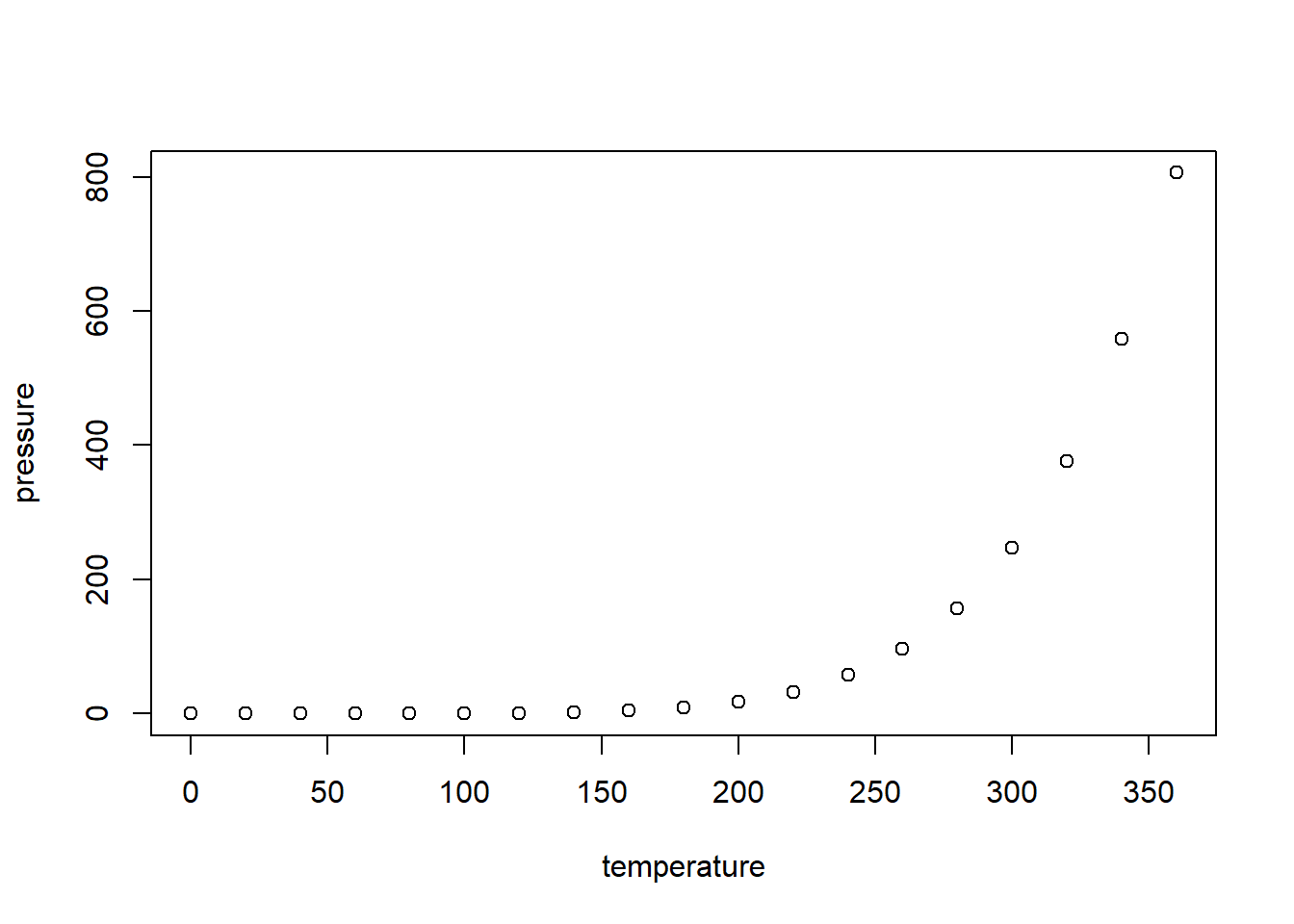
Including Plots
You can also embed plots, for example:
Note that the echo = FALSE parameter was added to the code chunk to prevent printing of the R code that generated the plot.