Final_Project

Online_Market_Clustering

Author

Tejaswini_Ketineni

Published

December 17, 2022

Objective

We have witnessed the emergence of many e-commerce companies in the past decade which has given rise to the surge of online retail sales.This indicates the way in which the process of shopping for the consumers has changed in time.During the earlier stages, people preferred going to a retail store and shop. But now since the way of shopping has transformed from more retail to more online, its mandatory to observe the certain key features: 1. The shopping process 2. The sites frequently visited 3. Payment information 4. Customer’s shopping address 5. Their internet activity etc.. A customer centric model for business is being built by the online websites to gain maximum profits This current project helps an online small business firm which sells unique gifts for all different occasions.The strategy which is employed by that particular store is that they opted to mail catalogues to the addresses.They procure orders through phone.The company has launched the website to go completely online.The main objective of this project is to help them understand the business behavioral pattern of the customers and to create a customer centric pattern.It is very much important to maintain the customer relation.

What is Customer Segmentation and it’s prospective use ?

Customer segmentation is the process in which we divide the groups based on the common characteristics.Our final goal is to find the customers who has the greatest potential to let the firm grow and retrieve maximum gains.The insights that we draw from the customer segmentation helps us design a proper segmentation strategy.Customer segmentation turns out beneficial for the following reasons :

1.We can devise a highly effective marketing strategy. 2.We can improve customer retention. 3.We can improve the metrics of conversion. 4.Enhanced product development.

Reading the Data

Loading required packages and data.

library(tibble)
library(dplyr)
library(ggplot2)
library(naniar)
library(tidyverse)
library(readr)
library(corpus)
library(tm)
library(tmap)
library(treemapify)
library(wordcloud)
library(dlookr)
library(highcharter)
library(countrycode)
knitr::opts_chunk$set(echo = TRUE, warning=FALSE, message=FALSE)

read the data extracted from kaggle which is from UCI machine learning repository.

#reading in the dataframe and checking the answers
Online_retail<-read.csv("_data/Online_Retail_v2.csv", header=TRUE)

head(Online_retail)

  Invoice    StockCode                Description Quantity    InvoiceDate
1 A563186            B            Adjust bad debt        1 12/08/11 14:51
2 A563187            B            Adjust bad debt        1 12/08/11 14:52
3  550193         PADS PADS TO MATCH ALL CUSHIONS        1  15/04/11 9:27
4  561226         PADS PADS TO MATCH ALL CUSHIONS        1 26/07/11 10:13
5  568200         PADS PADS TO MATCH ALL CUSHIONS        1 25/09/11 14:58
6  568375 BANK CHARGES               Bank Charges        1 26/09/11 17:01
   UnitPrice CustomerID        Country
1 -11062.060         NA United Kingdom
2 -11062.060         NA United Kingdom
3      0.001      13952 United Kingdom
4      0.001      15618 United Kingdom
5      0.001      16198 United Kingdom
6      0.001      13405 United Kingdom

df<-Online_retail

colnames(Online_retail)

[1] "Invoice"     "StockCode"   "Description" "Quantity"    "InvoiceDate"
[6] "UnitPrice"   "CustomerID"  "Country"

dim(Online_retail)

[1] 539394      8

The data set contains of about 539394 rows and 8 columns.

Cleaning the data and performing Feature Engineering.

miss_var_summary(Online_retail,order=TRUE)

# A tibble: 8 × 3
  variable    n_miss pct_miss
  <chr>        <int>    <dbl>
1 CustomerID  132605     24.6
2 Invoice          0      0  
3 StockCode        0      0  
4 Description      0      0  
5 Quantity         0      0  
6 InvoiceDate      0      0  
7 UnitPrice        0      0  
8 Country          0      0

gg_miss_var(Online_retail)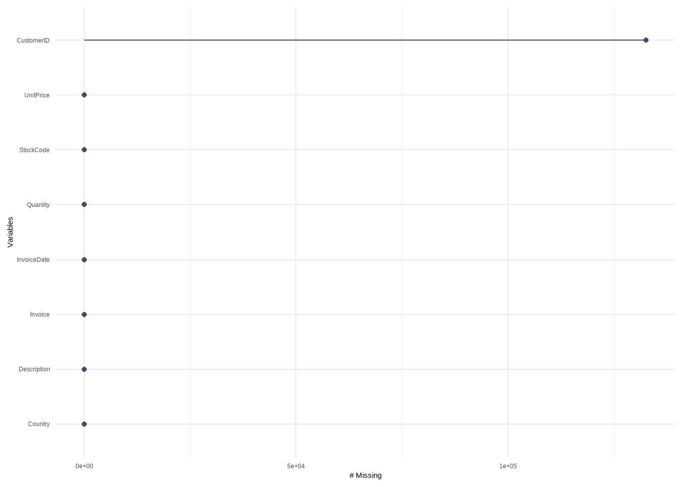

We see that the customer ID’s are missing we now see the structure of the whole data

summary(Online_retail)

   Invoice           StockCode         Description           Quantity        
 Length:539394      Length:539394      Length:539394      Min.   :-80995.00  
 Class :character   Class :character   Class :character   1st Qu.:     1.00  
 Mode  :character   Mode  :character   Mode  :character   Median :     3.00  
                                                          Mean   :     9.85  
                                                          3rd Qu.:    10.00  
                                                          Max.   : 80995.00  
                                                                             
 InvoiceDate          UnitPrice           CustomerID       Country         
 Length:539394      Min.   :-11062.06   Min.   :12346    Length:539394     
 Class :character   1st Qu.:     1.25   1st Qu.:13954    Class :character  
 Mode  :character   Median :     2.08   Median :15152    Mode  :character  
                    Mean   :     4.63   Mean   :15288                      
                    3rd Qu.:     4.13   3rd Qu.:16791                      
                    Max.   : 38970.00   Max.   :18287                      
                                        NA's   :132605

One notable observation we can see here is that the Quantity has negative value as minimum. we will look into this in further steps.

n_distinct(Online_retail$CustomerID)

[1] 4372

n_distinct(Online_retail$Description)

[1] 4042

sapply(Online_retail,function(x)sum(is.null(x)))

    Invoice   StockCode Description    Quantity InvoiceDate   UnitPrice 
          0           0           0           0           0           0 
 CustomerID     Country 
          0           0

sapply(Online_retail,function(x)sum(is.na(x)))

    Invoice   StockCode Description    Quantity InvoiceDate   UnitPrice 
          0           0           0           0           0           0 
 CustomerID     Country 
     132605           0

we see that there are 132605 missing values in CustomerID

Online_retail<-Online_retail%>%na.omit(Online_retail$CustomerID)
Online_retail$Description<-replace_na(Online_retail$Description, "No-info")

print(summarytools::dfSummary(Online_retail,varnumbers = FALSE,plain.ascii  = FALSE, 
                        style        = "grid", 
                        graph.magnif = 0.70, 
                        valid.col    = FALSE),
      method = 'render',
      table.classes = 'table-condensed')

Data Frame Summary

Online_retail

Dimensions: 406789 x 8
Duplicates: 5225

Variable

Stats / Values

Freqs (% of Valid)

Graph

Missing

Invoice [character]

1. 576339
2. 579196
3. 580727
4. 578270
5. 573576
6. 567656
7. 567183
8. 575607
9. 571441
10. 570488
[ 22176 others ]

542	(	0.1%	)
533	(	0.1%	)
529	(	0.1%	)
442	(	0.1%	)
435	(	0.1%	)
421	(	0.1%	)
399	(	0.1%	)
377	(	0.1%	)
364	(	0.1%	)
353	(	0.1%	)
402394	(	98.9%	)

0 (0.0%)

StockCode [character]

1. 85123A
2. 22423
3. 85099B
4. 84879
5. 47566
6. 20725
7. 22720
8. POST
9. 20727
10. 22197
[ 3674 others ]

2077	(	0.5%	)
1904	(	0.5%	)
1662	(	0.4%	)
1418	(	0.3%	)
1415	(	0.3%	)
1359	(	0.3%	)
1232	(	0.3%	)
1196	(	0.3%	)
1126	(	0.3%	)
1118	(	0.3%	)
392282	(	96.4%	)

0 (0.0%)

Description [character]

1. WHITE HANGING HEART T-LIG

2. REGENCY CAKESTAND 3 TIER

3. JUMBO BAG RED RETROSPOT

4. ASSORTED COLOUR BIRD ORNA

5. PARTY BUNTING

6. LUNCH BAG RED RETROSPOT

7. SET OF 3 CAKE TINS PANTRY

8. POSTAGE

9. LUNCH BAG BLACK SKULL.

10. PACK OF 72 RETROSPOT CAKE

[ 3886 others ]

2070	(	0.5%	)
1904	(	0.5%	)
1662	(	0.4%	)
1418	(	0.3%	)
1415	(	0.3%	)
1358	(	0.3%	)
1232	(	0.3%	)
1196	(	0.3%	)
1126	(	0.3%	)
1080	(	0.3%	)
392328	(	96.4%	)

0 (0.0%)

Quantity [integer]

Mean (sd) : 12 (247.9)

min ≤ med ≤ max:

-80995 ≤ 5 ≤ 80995

IQR (CV) : 10 (20.6)

435 distinct values

0 (0.0%)

InvoiceDate [character]

1. 14/11/11 15:27

2. 28/11/11 15:54

3. 05/12/11 17:17

4. 23/11/11 13:39

5. 31/10/11 14:09

6. 21/09/11 14:40

7. 10/11/11 12:37

8. 17/10/11 13:31

9. 10/10/11 17:12

10. 24/10/11 17:07

[ 20446 others ]

543	(	0.1%	)
534	(	0.1%	)
530	(	0.1%	)
444	(	0.1%	)
436	(	0.1%	)
422	(	0.1%	)
378	(	0.1%	)
365	(	0.1%	)
354	(	0.1%	)
353	(	0.1%	)
402430	(	98.9%	)

0 (0.0%)

UnitPrice [numeric]

Mean (sd) : 3.5 (69.3)

min ≤ med ≤ max:

0 ≤ 2 ≤ 38970

IQR (CV) : 2.5 (20)

619 distinct values

0 (0.0%)

CustomerID [integer]

Mean (sd) : 15287.8 (1713.6)

min ≤ med ≤ max:

12346 ≤ 15152 ≤ 18287

IQR (CV) : 2837 (0.1)

4371 distinct values

0 (0.0%)

Country [character]

1. United Kingdom

2. Germany

3. France

4. EIRE

5. Spain

6. Netherlands

7. Belgium

8. Switzerland

9. Portugal

10. Australia

[ 27 others ]

361854	(	89.0%	)
9493	(	2.3%	)
8490	(	2.1%	)
7483	(	1.8%	)
2532	(	0.6%	)
2367	(	0.6%	)
2069	(	0.5%	)
1876	(	0.5%	)
1480	(	0.4%	)
1256	(	0.3%	)
7889	(	1.9%	)

0 (0.0%)

Generated by summarytools 1.0.1 (R version 4.2.1)
2022-12-23

plot_outlier(Online_retail,UnitPrice,col="#AE4371")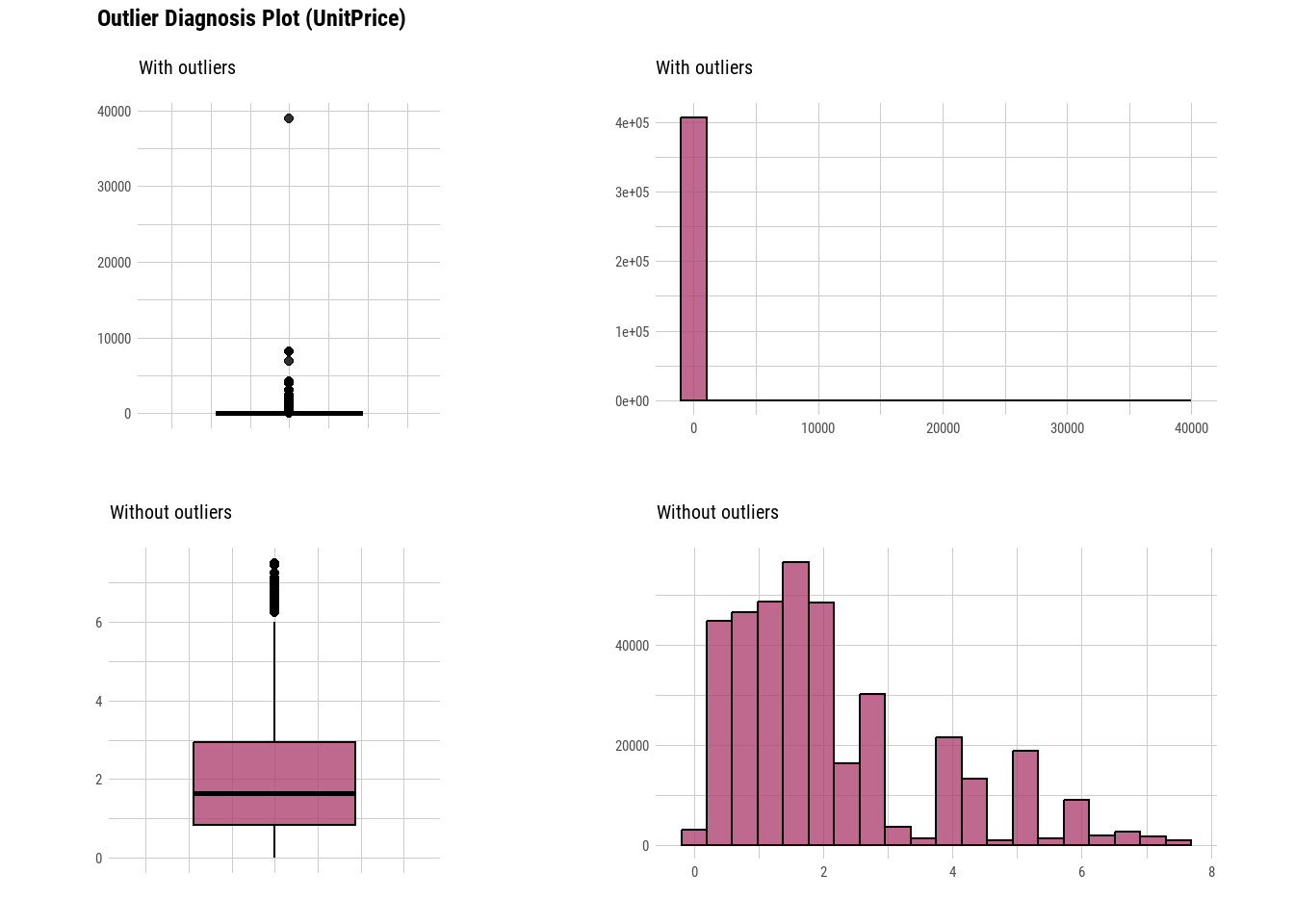

plot_outlier(Online_retail,Quantity,col="#E6AB02")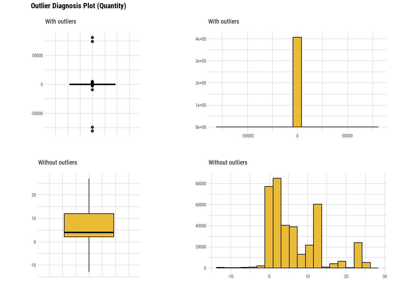

There are missing values present in CustomerID’s and if the description also has null values we replace the null values with “No info” and we simply omit the customerID.Data is highly skewed with outliers and when we remove them, it looks like normally distributed.

For quantity as we have seen above while calculating the summary, we see that there are negative values in the data. Instead of directly removing them as the outlier plot showed those values, there could be a possibility that negative and positive values of quantity could be inter-connected.To be elaborate, there is a high possibility that those outliers could be cancelled or reverted orders and hence got negative values.Let’s analyse in detail.

check_quantity<-Online_retail%>%filter(Quantity<0)

So we see a invoice charecter C , which could represent cancellation. Let’s sort this and understand the range.

check_quantity<-check_quantity%>%arrange(Quantity)

Let’s try to understand about the first listed entry to dig deep as it can be the huge outlier.We will study the orders made by the consumer with ID 16446.

Online_retail%>%filter(CustomerID==16446)

  Invoice StockCode                 Description Quantity   InvoiceDate
1  553573     22982         PANTRY PASTRY BRUSH        1 18/05/11 9:52
2  553573     22980      PANTRY SCRUBBING BRUSH        1 18/05/11 9:52
3 C581484     23843 PAPER CRAFT , LITTLE BIRDIE   -80995 09/12/11 9:27
4  581483     23843 PAPER CRAFT , LITTLE BIRDIE    80995 09/12/11 9:15
  UnitPrice CustomerID        Country
1      1.25      16446 United Kingdom
2      1.65      16446 United Kingdom
3      2.08      16446 United Kingdom
4      2.08      16446 United Kingdom

So we see that from the time stamps , PAPER CRAFT , LITTLE BIRDIE the order is cancelled in 12 mins after it is placed.So we remove all the cancelled orders.

Online_retail_no_outliers<-Online_retail%>%filter(Quantity>0)%>%filter(UnitPrice>0)

So, Now we have removed the outliers successfully.

FeatureEngineering.

In order to find out how much money is being spent, we come up with an idea of creating a variable called spent - which is a product of quantity and unit price.

Online_retail_new<-Online_retail_no_outliers%>%
  mutate(Online_retail_no_outliers,Expenditure=Quantity*UnitPrice)

colnames(Online_retail_new)

[1] "Invoice"     "StockCode"   "Description" "Quantity"    "InvoiceDate"
[6] "UnitPrice"   "CustomerID"  "Country"     "Expenditure"

We observe that the invoice date is in charecter variable type, So we would want to convert it to a date column.

library(lubridate)
Online_retail_new$InvoiceDate<-dmy_hm(Online_retail_new$InvoiceDate)
Online_retail_new$year<-year(Online_retail_new$InvoiceDate)
Online_retail_new$month<-month(Online_retail_new$InvoiceDate)
Online_retail_new$hour<-hour(Online_retail_new$InvoiceDate)
Online_retail_new$wday<-wday(Online_retail_new$InvoiceDate)

Exploratory Data Analysis Visualizations.

We first intend to understand the revenue generated by the countries to the firm.

dsub1<-Online_retail_new%>%group_by(Country) %>%dplyr::summarise(Total_Income = sum(Expenditure))
plot1 <- ggplot(dsub1,aes(x = reorder(Country,-Total_Income),Total_Income)) + geom_bar(stat = "identity",fill="dodgerblue2") + coord_flip()+  labs( x = 'Income_Earned',y = "Country", title = "Total Income by Country") +theme(axis.text.x = element_text(angle=90))
plot1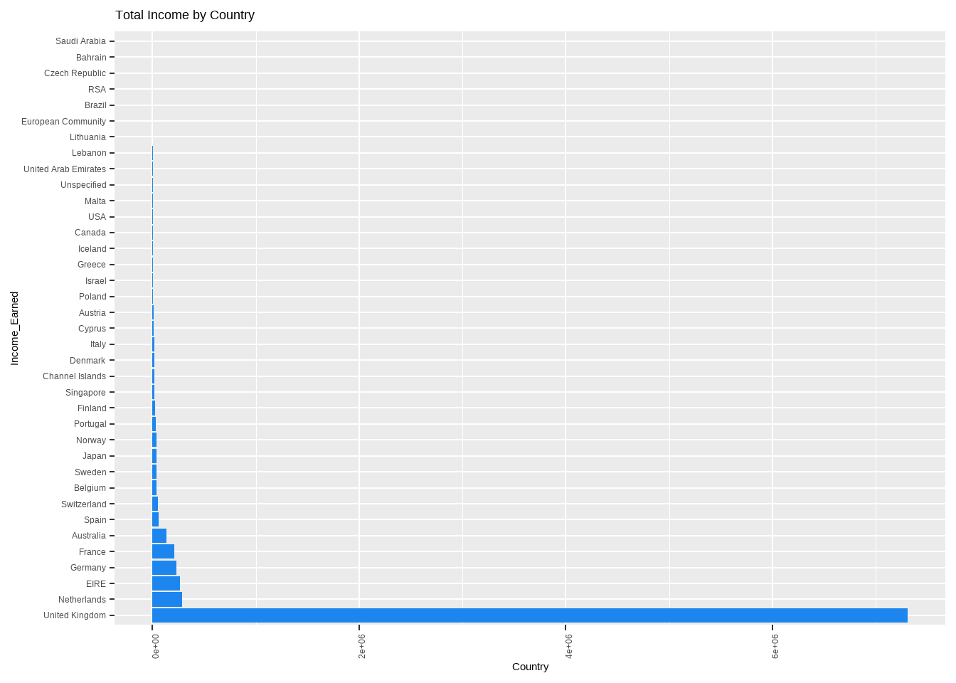

dsub2<-Online_retail_new %>%group_by(Country)%>%filter(Country!="United Kingdom")%>% 
dplyr::summarise(Total_Income = sum(Expenditure))

plot2<-ggplot(dsub2,aes(x = reorder(Country,-Total_Income),Total_Income)) + geom_bar(stat = "identity",fill="red") +  coord_flip()+ labs( x = 'Income_Earned',y = "Country", title = "Total Income by Country")+theme(axis.text.x = element_text(angle=90))
plot2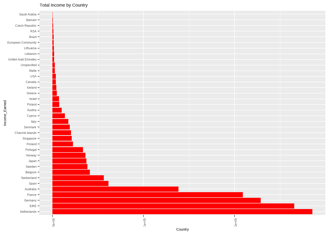

We see that there is huge revenue generated by united kingdom when compared to the other countries, and if we exclude UK, Netherlands has the highest share of Revenue.

library(ggplot2)
Revenue_by_month<-Online_retail_new%>% 
  group_by(month)%>%
  dplyr::summarise(Total_Income = sum(Expenditure))
plot_by_month<-ggplot(Revenue_by_month, mapping = aes(x = reorder(month, -Total_Income), Total_Income)) + 
  geom_bar(stat = "identity",fill="orchid4") +   labs( x = 'Revenue_generated',y = "Month", title = "Total Revenue by Month") +theme(axis.text.x = element_text(angle=90))

Revenue_by_year <- Online_retail_new %>% 
  group_by(year) %>% 
  dplyr::summarise(Total_Income = sum(Expenditure))
plot_by_year <- ggplot(Revenue_by_year, aes(x = reorder(year, -Total_Income), Total_Income)) + geom_bar(stat = "identity",fill="lightblue") +   labs( x = 'Revenue_generated',y = "year", title = "Total Revenue by year") +theme(axis.text.x = element_text(angle=90))

plot_by_month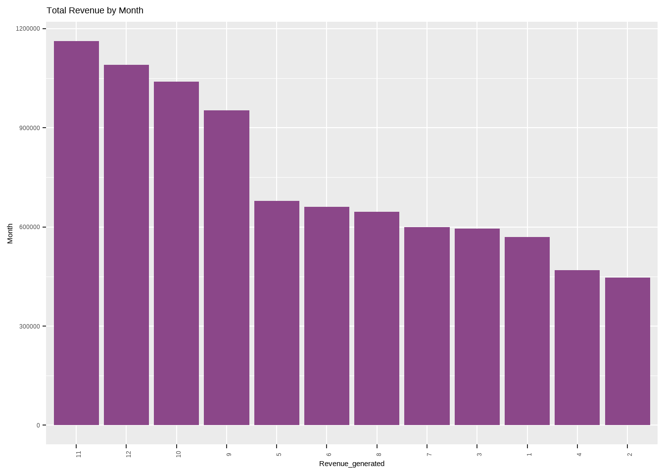

plot_by_year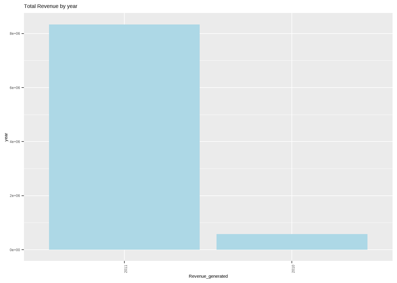

We observe that the month of november has the highest sales and the revenue generated has an exponential increase from 2010 to 2011. Now let us understand what are the items those are being frequently ordered and the items being frequently cancelled.

top_orders<-Online_retail_new %>% group_by(Description) %>% dplyr::summarise(Total_order_expense = sum(Expenditure)) %>% arrange(-Total_order_expense)
ggplot(data = head(top_orders,10),aes(x = reorder((Description), Total_order_expense), Total_order_expense)) + geom_bar(stat = "identity",fill="orange1")+  labs( y = 'Revenue',x = "Products", title = "Top 10 Products") +theme(axis.text.x = element_text(angle=90)) + coord_flip()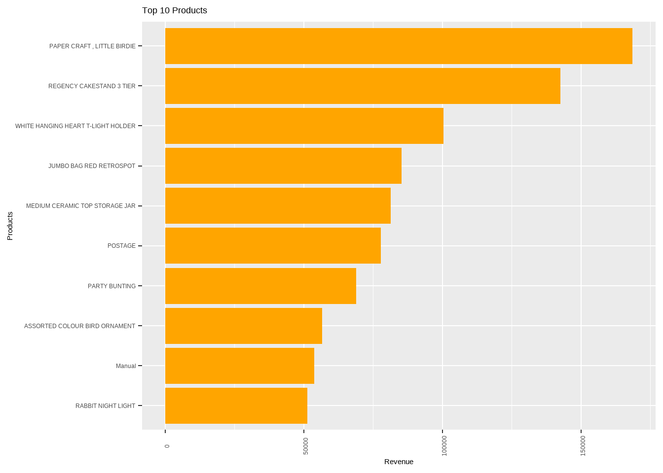

Tree graph representation of the same

top_orders<-Online_retail_new%>% group_by(Description)%>%dplyr::summarise(Total_order_expense = sum(Expenditure)) %>% arrange(-Total_order_expense)
ggplot(data = head(top_orders,10), aes(area = round(Total_order_expense,2), fill = Description,label=round(Total_order_expense,2))) +
  geom_treemap()+geom_treemap_text(colour = "black",place = "centre",size = 15)+scale_fill_brewer(palette = "Blues")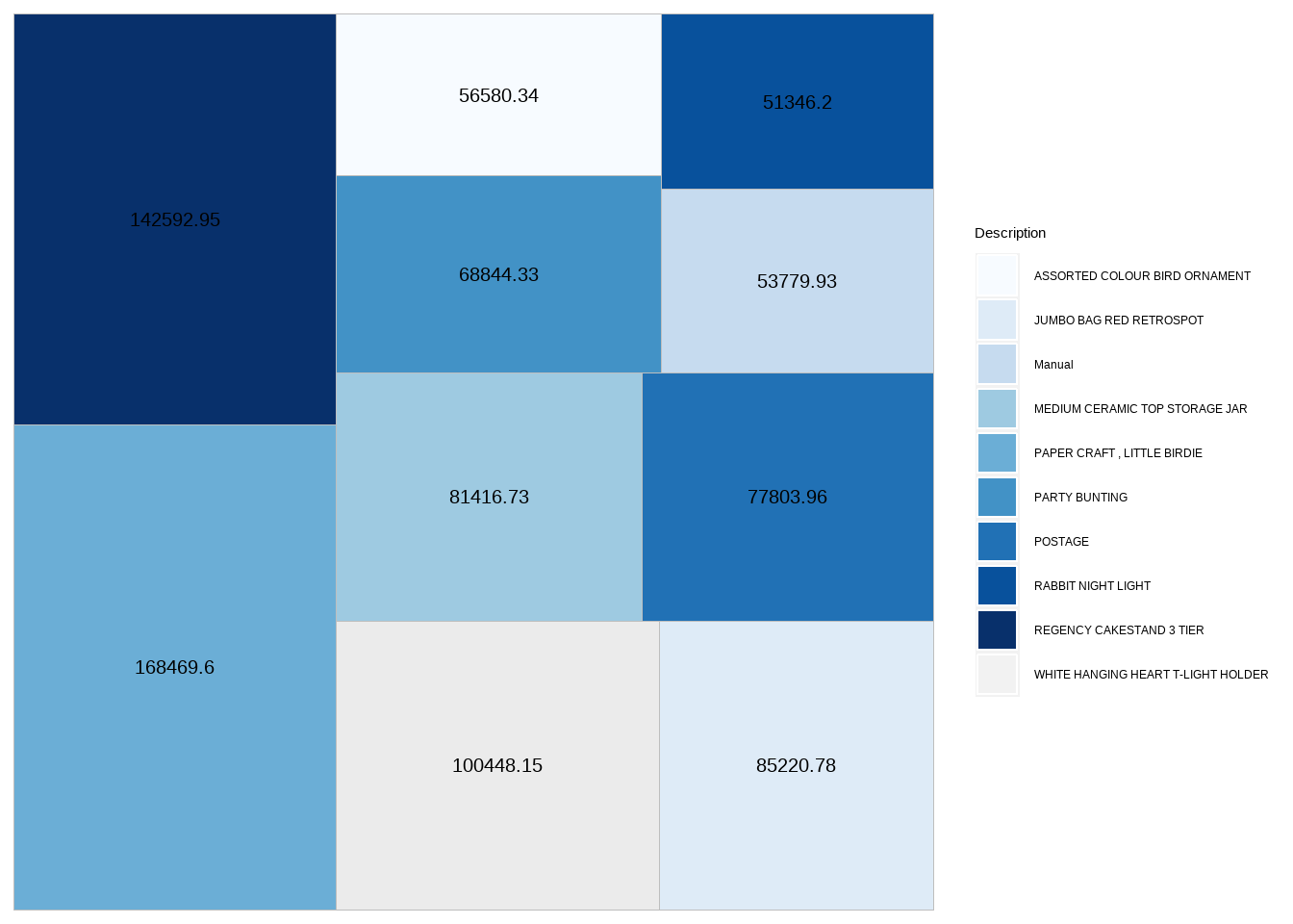

Now the cancelled metrics are understood and it is understood that paper craft, little birdie is cancelled as well along with being ordered more.

cancel_df<-Online_retail%>%filter(Quantity < 0)
cancel_df<-cancel_df%>%
  mutate(cancel_df,Expenditure=Quantity*UnitPrice)
cancelled_data <- cancel_df %>% group_by(Description) %>% dplyr::summarise(Total_order_expense = sum(Expenditure)) %>% arrange(Total_order_expense)
ggplot(head(cancelled_data,10),  aes(x = reorder((Description), -Total_order_expense), Total_order_expense)) + geom_bar(stat = "identity",fill="turquoise4")+  labs( y = 'Income',x = "Products", title = "Top 10 Products- cancelled") +theme(axis.text.x = element_text(angle=90)) + coord_flip()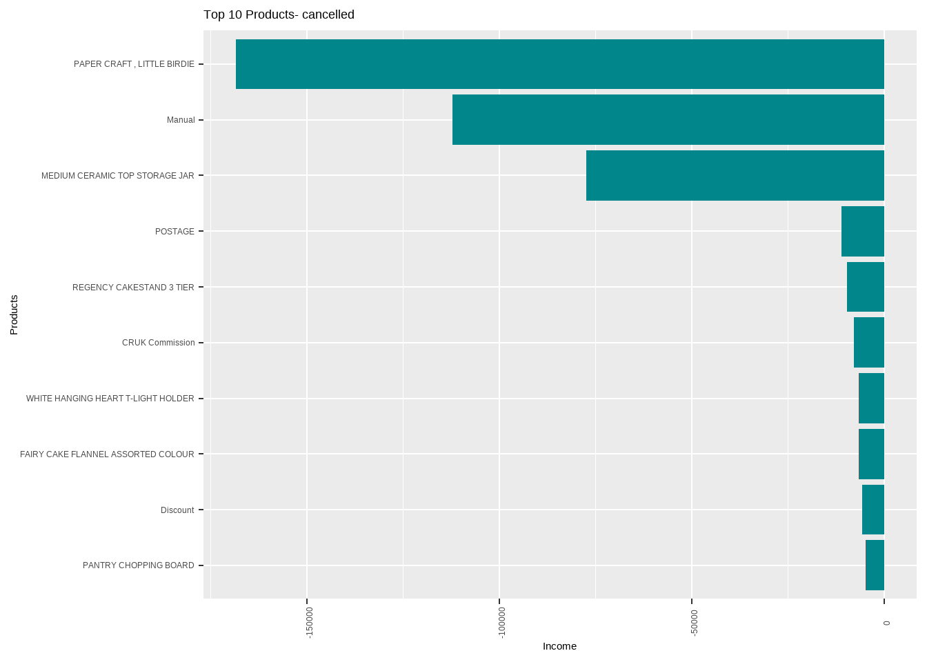

We now are going to understand the unique words in the description, which are observed in the orders.

products_list <- unique(Online_retail_new$Description)
p_list <- Corpus(VectorSource(products_list))
toSpace <- content_transformer(function (x , pattern) gsub(pattern, " ", x))
p_list<-tm_map(p_list, toSpace, "/")
p_list<-tm_map(p_list, toSpace, "@")
p_list<-tm_map(p_list, toSpace, "\\|")
p_list<-tm_map(p_list, content_transformer(tolower))
p_list<-tm_map(p_list, removeNumbers)
p_list<-tm_map(p_list, removeWords, stopwords("english"))
p_list<-tm_map(p_list, removeWords, c( "blue","white","metal","small", "large","red","black","design","pink","glass","set"))
p_list<-tm_map(p_list, removePunctuation)
p_list<-tm_map(p_list, stripWhitespace)
dtm<-TermDocumentMatrix(p_list)
m<-as.matrix(dtm)
v<-sort(rowSums(m),decreasing=TRUE)
d<-data.frame(word = names(v),freq=v)

set.seed(123)
wordcloud(words=d$word,freq=d$freq,min.freq=1,
          max.words=20, random.order=FALSE, rot.per=0.35, 
          colors=brewer.pal(8,"Dark2"))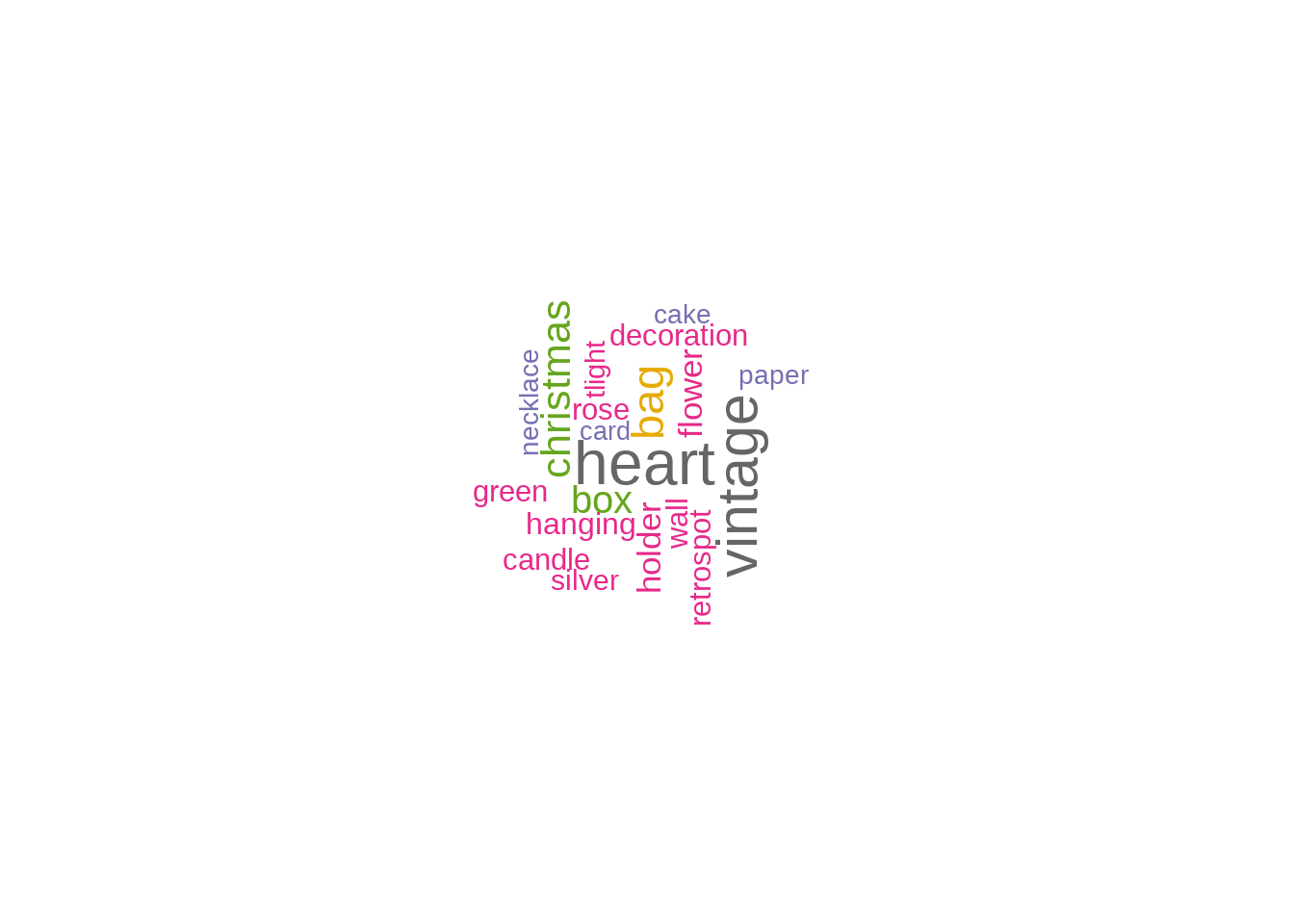

A bigger font size usually represents higher repetition of that particular word in description.The stop words are chosen iteratively because the colors would not give any useful insights while studying the frequently ordered item.

world_map<-Online_retail_new%>%group_by(Country)%>% dplyr::summarise(revenue=sum(Expenditure))
  
highchart(type = "map") %>%hc_add_series_map(worldgeojson,world_map%>%bind_cols(as_tibble(world_map$revenue)) %>% group_by(world_map$Country) %>% dplyr::summarise(revenue = log1p(sum(value))) %>% ungroup() %>% mutate(iso2 = countrycode(sourcevar = world_map$Country,origin="country.name", destination="iso2c")),value = "revenue", joinBy = "iso2") %>%
hc_title(text = "Revenue by country (log)") %>%
hc_tooltip(useHTML = TRUE, headerFormat = "",pointFormat = "{point.map_info$Country}") %>% 
  hc_colorAxis(stops = color_stops(colors = viridisLite::inferno(10, begin = 0.1)))

summary(Online_retail_new)

   Invoice           StockCode         Description           Quantity       
 Length:397884      Length:397884      Length:397884      Min.   :    1.00  
 Class :character   Class :character   Class :character   1st Qu.:    2.00  
 Mode  :character   Mode  :character   Mode  :character   Median :    6.00  
                                                          Mean   :   12.99  
                                                          3rd Qu.:   12.00  
                                                          Max.   :80995.00  
  InvoiceDate                       UnitPrice          CustomerID   
 Min.   :2010-12-01 08:26:00.00   Min.   :   0.001   Min.   :12346  
 1st Qu.:2011-04-07 11:12:00.00   1st Qu.:   1.250   1st Qu.:13969  
 Median :2011-07-31 14:39:00.00   Median :   1.950   Median :15159  
 Mean   :2011-07-10 23:41:23.50   Mean   :   3.116   Mean   :15294  
 3rd Qu.:2011-10-20 14:33:00.00   3rd Qu.:   3.750   3rd Qu.:16795  
 Max.   :2011-12-09 12:50:00.00   Max.   :8142.750   Max.   :18287  
   Country           Expenditure             year          month       
 Length:397884      Min.   :     0.00   Min.   :2010   Min.   : 1.000  
 Class :character   1st Qu.:     4.68   1st Qu.:2011   1st Qu.: 5.000  
 Mode  :character   Median :    11.80   Median :2011   Median : 8.000  
                    Mean   :    22.40   Mean   :2011   Mean   : 7.612  
                    3rd Qu.:    19.80   3rd Qu.:2011   3rd Qu.:11.000  
                    Max.   :168469.60   Max.   :2011   Max.   :12.000  
      hour            wday     
 Min.   : 6.00   Min.   :1.00  
 1st Qu.:11.00   1st Qu.:2.00  
 Median :13.00   Median :4.00  
 Mean   :12.73   Mean   :3.51  
 3rd Qu.:14.00   3rd Qu.:5.00  
 Max.   :20.00   Max.   :6.00

As we know, the clustering is grouping homogenous data points together.The motive of clustering is to make the Distance between data points in the cluster should be made minimal.we adopt a variety of clustering algorithms and RFM analysis is one of the most pivotal step. RFM Analysis gives score to each of the customers on three elements of recency, frequency and monetary. The lesser value of recency depicts that the customer visits the store more.Frequency depicts the gap between two purchases and higher value indicates more frequent purchases.Monetary refers to the amount of money spent.

recency<-Online_retail_new%>%dplyr::select(CustomerID,InvoiceDate)%>%mutate(recency= as.Date("2011-12-09")-as.Date(InvoiceDate))  
recency<-recency%>%dplyr::select(CustomerID,recency)%>%group_by(CustomerID)%>% slice(which.min(recency))

#frequency
amount_products<-Online_retail_new%>%dplyr::select(CustomerID,InvoiceDate)%>%group_by(CustomerID, InvoiceDate)%>%dplyr::summarise(n_prod=n())
df_frequency<-amount_products %>% dplyr::select(CustomerID) %>%group_by(CustomerID) %>% dplyr::summarise(frequency=n())

#monetary
customer<-summarise_at(group_by(Online_retail_new,CustomerID,Country), vars(Expenditure,Quantity), funs(sum(.,na.rm = TRUE)))
monetary<-select(customer, c("CustomerID", "Expenditure"))

#RFM DF
# inner join the three RFM data frames by CustomerID
rfm<-recency%>%dplyr::inner_join(., df_frequency, by = "CustomerID") %>% dplyr::inner_join(., monetary, by = "CustomerID")
# drop the days from recency column and transform it into numeric data type
rfm<-rfm %>% mutate(recency=str_replace(recency, " days", "")) %>% mutate(recency = as.numeric(recency)) %>% ungroup()
head(rfm, 3)

# A tibble: 3 × 4
  CustomerID recency frequency Expenditure
       <int>   <dbl>     <int>       <dbl>
1      12346     325         1      77184.
2      12347       2         7       4310 
3      12348      75         4       1797.

we now scale the data frame.

rfm1<-select(rfm,-CustomerID)
df_scale<-scale(rfm1)

Now we use silhouette method to find out optimal number of clusters.

library(factoextra)
fviz_nbclust(df_scale, kmeans,method="silhouette")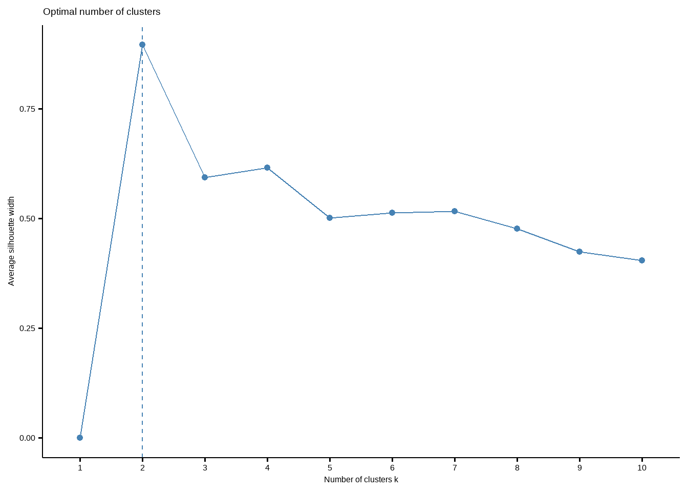

We now perform kmeans clustering with optimal clusters

set.seed(123)
k_means_clustering<- kmeans(df_scale, 2, nstart = 25)
fviz_cluster(k_means_clustering,df_scale)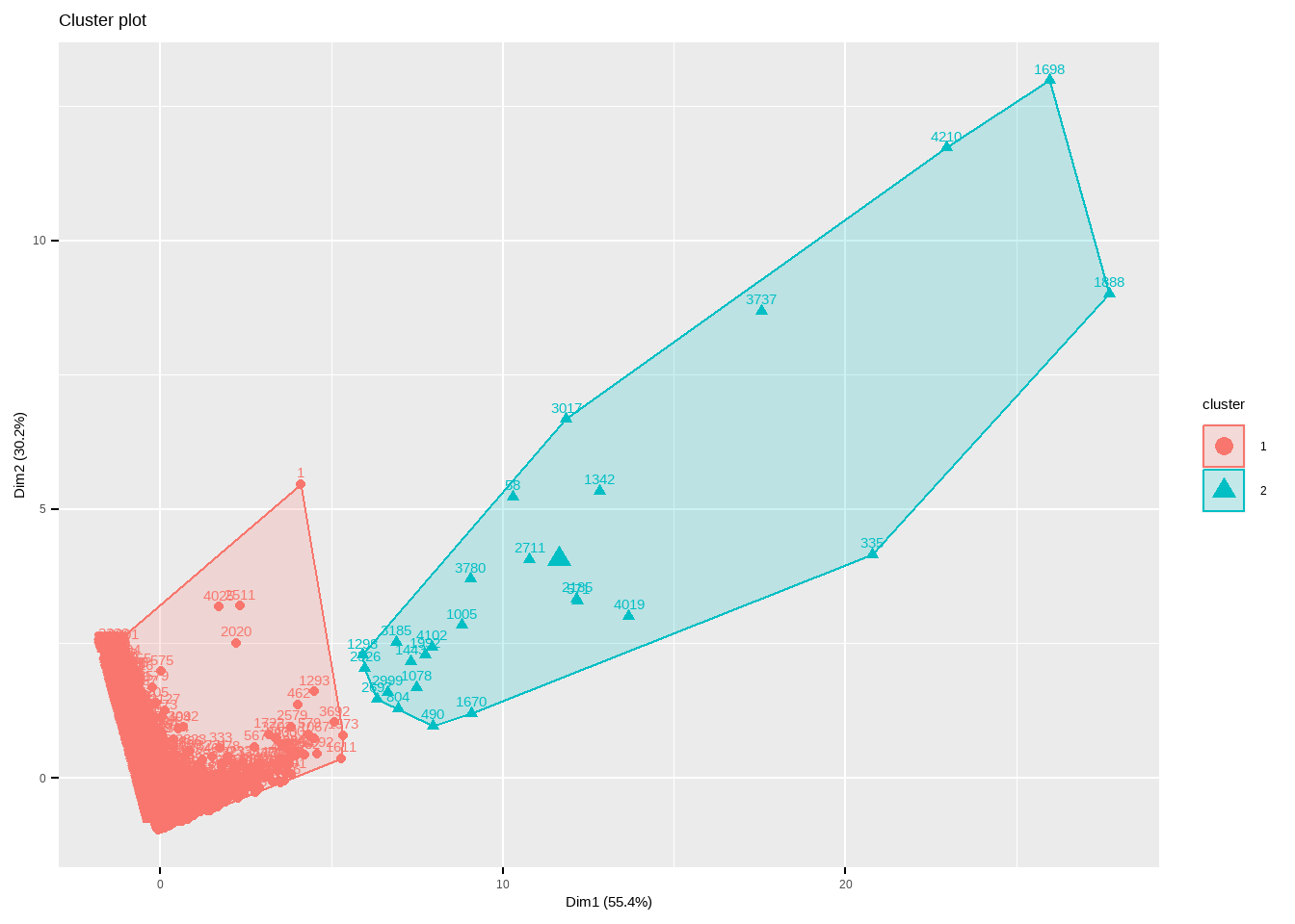

print(k_means_clustering)

K-means clustering with 2 clusters of sizes 4320, 26

Cluster means:
       recency frequency Expenditure
1  0.005210046 -0.048307 -0.05619323
2 -0.865669143  8.026394  9.33672099

Clustering vector:
   [1] 1 1 1 1 1 1 1 1 1 1 1 1 1 1 1 1 1 1 1 1 1 1 1 1 1 1 1 1 1 1 1 1 1 1 1 1 1
  [38] 1 1 1 1 1 1 1 1 1 1 1 1 1 1 1 1 1 1 1 1 2 1 1 1 1 1 1 1 1 1 1 1 1 1 1 1 1
  [75] 1 1 1 1 1 1 1 1 1 1 1 1 1 1 1 1 1 1 1 1 1 1 1 1 1 1 1 1 1 1 1 1 1 1 1 1 1
 [112] 1 1 1 1 1 1 1 1 1 1 1 1 1 1 1 1 1 1 1 1 1 1 1 1 1 1 1 1 1 1 1 1 1 1 1 1 1
 [149] 1 1 1 1 1 1 1 1 1 1 1 1 1 1 1 1 1 1 1 1 1 1 1 1 1 1 1 1 1 1 1 1 1 1 1 1 1
 [186] 1 1 1 1 1 1 1 1 1 1 1 1 1 1 1 1 1 1 1 1 1 1 1 1 1 1 1 1 1 1 1 1 1 1 1 1 1
 [223] 1 1 1 1 1 1 1 1 1 1 1 1 1 1 1 1 1 1 1 1 1 1 1 1 1 1 1 1 1 1 1 1 1 1 1 1 1
 [260] 1 1 1 1 1 1 1 1 1 1 1 1 1 1 1 1 1 1 1 1 1 1 1 1 1 1 1 1 1 1 1 1 1 1 1 1 1
 [297] 1 1 1 1 1 1 1 1 1 1 1 1 1 1 1 1 1 1 1 1 1 1 1 1 1 1 1 1 1 1 1 1 1 1 1 1 1
 [334] 1 2 1 1 1 1 1 1 1 1 1 1 1 1 1 1 1 1 1 1 1 1 1 1 1 1 1 1 1 1 1 1 1 1 1 1 1
 [371] 1 1 1 1 1 1 1 1 1 1 1 1 1 1 1 1 1 1 1 1 1 1 1 1 1 1 1 1 1 1 1 1 1 1 1 1 1
 [408] 1 1 1 1 1 1 1 1 1 1 1 1 1 1 1 1 1 1 1 1 1 1 1 1 1 1 1 1 1 1 1 1 1 1 1 1 1
 [445] 1 1 1 1 1 1 1 1 1 1 1 1 1 1 1 1 1 1 1 1 1 1 1 1 1 1 1 1 1 1 1 1 1 1 1 1 1
 [482] 1 1 1 1 1 1 1 1 2 1 1 1 1 1 1 1 1 1 1 1 1 1 1 1 1 1 1 1 1 1 1 1 1 1 1 1 1
 [519] 1 1 1 1 1 1 1 1 1 1 1 1 1 1 1 1 1 1 1 1 1 1 1 1 1 1 1 1 1 1 1 1 1 1 1 1 1
 [556] 1 1 1 1 1 1 1 1 1 1 1 1 1 1 1 2 1 1 1 1 1 1 1 1 1 1 1 1 1 1 1 1 1 1 1 1 1
 [593] 1 1 1 1 1 1 1 1 1 1 1 1 1 1 1 1 1 1 1 1 1 1 1 1 1 1 1 1 1 1 1 1 1 1 1 1 1
 [630] 1 1 1 1 1 1 1 1 1 1 1 1 1 1 1 1 1 1 1 1 1 1 1 1 1 1 1 1 1 1 1 1 1 1 1 1 1
 [667] 1 1 1 1 1 1 1 1 1 1 1 1 1 1 1 1 1 1 1 1 1 1 1 1 1 1 1 1 1 1 1 1 1 1 1 1 1
 [704] 1 1 1 1 1 1 1 1 1 1 1 1 1 1 1 1 1 1 1 1 1 1 1 1 1 1 1 1 1 1 1 1 1 1 1 1 1
 [741] 1 1 1 1 1 1 1 1 1 1 1 1 1 1 1 1 1 1 1 1 1 1 1 1 1 1 1 1 1 1 1 1 1 1 1 1 1
 [778] 1 1 1 1 1 1 1 1 1 1 1 1 1 1 1 1 1 1 1 1 1 1 1 1 1 1 2 1 1 1 1 1 1 1 1 1 1
 [815] 1 1 1 1 1 1 1 1 1 1 1 1 1 1 1 1 1 1 1 1 1 1 1 1 1 1 1 1 1 1 1 1 1 1 1 1 1
 [852] 1 1 1 1 1 1 1 1 1 1 1 1 1 1 1 1 1 1 1 1 1 1 1 1 1 1 1 1 1 1 1 1 1 1 1 1 1
 [889] 1 1 1 1 1 1 1 1 1 1 1 1 1 1 1 1 1 1 1 1 1 1 1 1 1 1 1 1 1 1 1 1 1 1 1 1 1
 [926] 1 1 1 1 1 1 1 1 1 1 1 1 1 1 1 1 1 1 1 1 1 1 1 1 1 1 1 1 1 1 1 1 1 1 1 1 1
 [963] 1 1 1 1 1 1 1 1 1 1 1 1 1 1 1 1 1 1 1 1 1 1 1 1 1 1 1 1 1 1 1 1 1 1 1 1 1
[1000] 1 1 1 1 1 2 1 1 1 1 1 1 1 1 1 1 1 1 1 1 1 1 1 1 1 1 1 1 1 1 1 1 1 1 1 1 1
[1037] 1 1 1 1 1 1 1 1 1 1 1 1 1 1 1 1 1 1 1 1 1 1 1 1 1 1 1 1 1 1 1 1 1 1 1 1 1
[1074] 1 1 1 1 2 1 1 1 1 1 1 1 1 1 1 1 1 1 1 1 1 1 1 1 1 1 1 1 1 1 1 1 1 1 1 1 1
[1111] 1 1 1 1 1 1 1 1 1 1 1 1 1 1 1 1 1 1 1 1 1 1 1 1 1 1 1 1 1 1 1 1 1 1 1 1 1
[1148] 1 1 1 1 1 1 1 1 1 1 1 1 1 1 1 1 1 1 1 1 1 1 1 1 1 1 1 1 1 1 1 1 1 1 1 1 1
[1185] 1 1 1 1 1 1 1 1 1 1 1 1 1 1 1 1 1 1 1 1 1 1 1 1 1 1 1 1 1 1 1 1 1 1 1 1 1
[1222] 1 1 1 1 1 1 1 1 1 1 1 1 1 1 1 1 1 1 1 1 1 1 1 1 1 1 1 1 1 1 1 1 1 1 1 1 1
[1259] 1 1 1 1 1 1 1 1 1 1 1 1 1 1 1 1 1 1 1 1 1 1 1 1 1 1 1 1 1 1 1 1 1 1 1 1 1
[1296] 1 1 2 1 1 1 1 1 1 1 1 1 1 1 1 1 1 1 1 1 1 1 1 1 1 1 1 1 1 1 1 1 1 1 1 1 1
[1333] 1 1 1 1 1 1 1 1 1 2 1 1 1 1 1 1 1 1 1 1 1 1 1 1 1 1 1 1 1 1 1 1 1 1 1 1 1
[1370] 1 1 1 1 1 1 1 1 1 1 1 1 1 1 1 1 1 1 1 1 1 1 1 1 1 1 1 1 1 1 1 1 1 1 1 1 1
[1407] 1 1 1 1 1 1 1 1 1 1 1 1 1 1 1 1 1 1 1 1 1 1 1 1 1 1 1 1 1 1 1 1 1 1 1 1 2
[1444] 1 1 1 1 1 1 1 1 1 1 1 1 1 1 1 1 1 1 1 1 1 1 1 1 1 1 1 1 1 1 1 1 1 1 1 1 1
[1481] 1 1 1 1 1 1 1 1 1 1 1 1 1 1 1 1 1 1 1 1 1 1 1 1 1 1 1 1 1 1 1 1 1 1 1 1 1
[1518] 1 1 1 1 1 1 1 1 1 1 1 1 1 1 1 1 1 1 1 1 1 1 1 1 1 1 1 1 1 1 1 1 1 1 1 1 1
[1555] 1 1 1 1 1 1 1 1 1 1 1 1 1 1 1 1 1 1 1 1 1 1 1 1 1 1 1 1 1 1 1 1 1 1 1 1 1
[1592] 1 1 1 1 1 1 1 1 1 1 1 1 1 1 1 1 1 1 1 1 1 1 1 1 1 1 1 1 1 1 1 1 1 1 1 1 1
[1629] 1 1 1 1 1 1 1 1 1 1 1 1 1 1 1 1 1 1 1 1 1 1 1 1 1 1 1 1 1 1 1 1 1 1 1 1 1
[1666] 1 1 1 1 2 1 1 1 1 1 1 1 1 1 1 1 1 1 1 1 1 1 1 1 1 1 1 1 1 1 1 1 2 1 1 1 1
[1703] 1 1 1 1 1 1 1 1 1 1 1 1 1 1 1 1 1 1 1 1 1 1 1 1 1 1 1 1 1 1 1 1 1 1 1 1 1
[1740] 1 1 1 1 1 1 1 1 1 1 1 1 1 1 1 1 1 1 1 1 1 1 1 1 1 1 1 1 1 1 1 1 1 1 1 1 1
[1777] 1 1 1 1 1 1 1 1 1 1 1 1 1 1 1 1 1 1 1 1 1 1 1 1 1 1 1 1 1 1 1 1 1 1 1 1 1
[1814] 1 1 1 1 1 1 1 1 1 1 1 1 1 1 1 1 1 1 1 1 1 1 1 1 1 1 1 1 1 1 1 1 1 1 1 1 1
[1851] 1 1 1 1 1 1 1 1 1 1 1 1 1 1 1 1 1 1 1 1 1 1 1 1 1 1 1 1 1 1 1 1 1 1 1 1 1
[1888] 2 1 1 1 1 1 1 1 1 1 1 1 1 1 1 1 1 1 1 1 1 1 1 1 1 1 1 1 1 1 1 1 1 1 1 1 1
[1925] 1 1 1 1 1 1 1 1 1 1 1 1 1 1 1 1 1 1 1 1 1 1 1 1 1 1 1 1 1 1 1 1 1 1 1 1 1
[1962] 1 1 1 1 1 1 1 1 1 1 1 1 1 1 1 1 1 1 1 1 1 1 1 1 1 1 1 1 1 1 2 1 1 1 1 1 1
[1999] 1 1 1 1 1 1 1 1 1 1 1 1 1 1 1 1 1 1 1 1 1 1 1 1 1 1 1 1 1 1 1 1 1 1 1 1 1
[2036] 1 1 1 1 1 1 1 1 1 1 1 1 1 1 1 1 1 1 1 1 1 1 1 1 1 1 1 1 1 1 1 1 1 1 1 1 1
[2073] 1 1 1 1 1 1 1 1 1 1 1 1 1 1 1 1 1 1 1 1 1 1 1 1 1 1 1 1 1 1 1 1 1 1 1 1 1
[2110] 1 1 1 1 1 1 1 1 1 1 1 1 1 1 1 1 1 1 1 1 1 1 1 1 1 1 1 1 1 1 1 1 1 1 1 1 1
[2147] 1 1 1 1 1 1 1 1 1 1 1 1 1 1 1 1 1 1 1 1 1 1 1 1 1 1 1 1 1 1 1 1 1 1 1 1 1
[2184] 1 2 1 1 1 1 1 1 1 1 1 1 1 1 1 1 1 1 1 1 1 1 1 1 1 1 1 1 1 1 1 1 1 1 1 1 1
[2221] 1 1 1 1 1 1 1 1 1 1 1 1 1 1 1 1 1 1 1 1 1 1 1 1 1 1 1 1 1 1 1 1 1 1 1 1 1
[2258] 1 1 1 1 1 1 1 1 1 1 1 1 1 1 1 1 1 1 1 1 1 1 1 1 1 1 1 1 1 1 1 1 1 1 1 1 1
[2295] 1 1 1 1 1 1 1 1 1 1 1 1 1 1 1 1 1 1 1 1 1 1 1 1 1 1 1 1 1 1 1 1 1 1 1 1 1
[2332] 1 1 1 1 1 1 1 1 1 1 1 1 1 1 1 1 1 1 1 1 1 1 1 1 1 1 1 1 1 1 1 1 1 1 1 1 1
[2369] 1 1 1 1 1 1 1 1 1 1 1 1 1 1 1 1 1 1 1 1 1 1 1 1 1 1 1 1 1 1 1 1 1 1 1 1 1
[2406] 1 1 1 1 1 1 1 1 1 1 1 1 1 1 1 1 1 1 1 1 1 1 1 1 1 1 1 1 1 1 1 1 1 1 1 1 1
[2443] 1 1 1 1 1 1 1 1 1 1 1 1 1 1 1 1 1 1 1 1 1 1 1 1 1 1 1 1 1 1 1 1 1 1 1 1 1
[2480] 1 1 1 1 1 1 1 1 1 1 1 1 1 1 1 1 1 1 1 1 1 1 1 1 1 1 1 1 1 1 1 1 1 1 1 1 1
[2517] 1 1 1 1 1 1 1 1 1 2 1 1 1 1 1 1 1 1 1 1 1 1 1 1 1 1 1 1 1 1 1 1 1 1 1 1 1
[2554] 1 1 1 1 1 1 1 1 1 1 1 1 1 1 1 1 1 1 1 1 1 1 1 1 1 1 1 1 1 1 1 1 1 1 1 1 1
[2591] 1 1 1 1 1 1 1 1 1 1 1 1 1 1 1 1 1 1 1 1 1 1 1 1 1 1 1 1 1 1 1 1 1 1 1 1 1
[2628] 1 1 1 1 1 1 1 1 1 1 1 1 1 1 1 1 1 1 1 1 1 1 1 1 1 1 1 1 1 1 1 1 1 1 1 1 1
[2665] 1 1 1 1 1 1 1 1 1 1 1 1 1 1 1 1 1 1 1 1 1 1 1 1 1 1 1 1 1 1 1 1 2 1 1 1 1
[2702] 1 1 1 1 1 1 1 1 1 2 1 1 1 1 1 1 1 1 1 1 1 1 1 1 1 1 1 1 1 1 1 1 1 1 1 1 1
[2739] 1 1 1 1 1 1 1 1 1 1 1 1 1 1 1 1 1 1 1 1 1 1 1 1 1 1 1 1 1 1 1 1 1 1 1 1 1
[2776] 1 1 1 1 1 1 1 1 1 1 1 1 1 1 1 1 1 1 1 1 1 1 1 1 1 1 1 1 1 1 1 1 1 1 1 1 1
[2813] 1 1 1 1 1 1 1 1 1 1 1 1 1 1 1 1 1 1 1 1 1 1 1 1 1 1 1 1 1 1 1 1 1 1 1 1 1
[2850] 1 1 1 1 1 1 1 1 1 1 1 1 1 1 1 1 1 1 1 1 1 1 1 1 1 1 1 1 1 1 1 1 1 1 1 1 1
[2887] 1 1 1 1 1 1 1 1 1 1 1 1 1 1 1 1 1 1 1 1 1 1 1 1 1 1 1 1 1 1 1 1 1 1 1 1 1
[2924] 1 1 1 1 1 1 1 1 1 1 1 1 1 1 1 1 1 1 1 1 1 1 1 1 1 1 1 1 1 1 1 1 1 1 1 1 1
[2961] 1 1 1 1 1 1 1 1 1 1 1 1 1 1 1 1 1 1 1 1 1 1 1 1 1 1 1 1 1 1 1 1 1 1 1 1 1
[2998] 1 2 1 1 1 1 1 1 1 1 1 1 1 1 1 1 1 1 1 2 1 1 1 1 1 1 1 1 1 1 1 1 1 1 1 1 1
[3035] 1 1 1 1 1 1 1 1 1 1 1 1 1 1 1 1 1 1 1 1 1 1 1 1 1 1 1 1 1 1 1 1 1 1 1 1 1
[3072] 1 1 1 1 1 1 1 1 1 1 1 1 1 1 1 1 1 1 1 1 1 1 1 1 1 1 1 1 1 1 1 1 1 1 1 1 1
[3109] 1 1 1 1 1 1 1 1 1 1 1 1 1 1 1 1 1 1 1 1 1 1 1 1 1 1 1 1 1 1 1 1 1 1 1 1 1
[3146] 1 1 1 1 1 1 1 1 1 1 1 1 1 1 1 1 1 1 1 1 1 1 1 1 1 1 1 1 1 1 1 1 1 1 1 1 1
[3183] 1 1 2 1 1 1 1 1 1 1 1 1 1 1 1 1 1 1 1 1 1 1 1 1 1 1 1 1 1 1 1 1 1 1 1 1 1
[3220] 1 1 1 1 1 1 1 1 1 1 1 1 1 1 1 1 1 1 1 1 1 1 1 1 1 1 1 1 1 1 1 1 1 1 1 1 1
[3257] 1 1 1 1 1 1 1 1 1 1 1 1 1 1 1 1 1 1 1 1 1 1 1 1 1 1 1 1 1 1 1 1 1 1 1 1 1
[3294] 1 1 1 1 1 1 1 1 1 1 1 1 1 1 1 1 1 1 1 1 1 1 1 1 1 1 1 1 1 1 1 1 1 1 1 1 1
[3331] 1 1 1 1 1 1 1 1 1 1 1 1 1 1 1 1 1 1 1 1 1 1 1 1 1 1 1 1 1 1 1 1 1 1 1 1 1
[3368] 1 1 1 1 1 1 1 1 1 1 1 1 1 1 1 1 1 1 1 1 1 1 1 1 1 1 1 1 1 1 1 1 1 1 1 1 1
[3405] 1 1 1 1 1 1 1 1 1 1 1 1 1 1 1 1 1 1 1 1 1 1 1 1 1 1 1 1 1 1 1 1 1 1 1 1 1
[3442] 1 1 1 1 1 1 1 1 1 1 1 1 1 1 1 1 1 1 1 1 1 1 1 1 1 1 1 1 1 1 1 1 1 1 1 1 1
[3479] 1 1 1 1 1 1 1 1 1 1 1 1 1 1 1 1 1 1 1 1 1 1 1 1 1 1 1 1 1 1 1 1 1 1 1 1 1
[3516] 1 1 1 1 1 1 1 1 1 1 1 1 1 1 1 1 1 1 1 1 1 1 1 1 1 1 1 1 1 1 1 1 1 1 1 1 1
[3553] 1 1 1 1 1 1 1 1 1 1 1 1 1 1 1 1 1 1 1 1 1 1 1 1 1 1 1 1 1 1 1 1 1 1 1 1 1
[3590] 1 1 1 1 1 1 1 1 1 1 1 1 1 1 1 1 1 1 1 1 1 1 1 1 1 1 1 1 1 1 1 1 1 1 1 1 1
[3627] 1 1 1 1 1 1 1 1 1 1 1 1 1 1 1 1 1 1 1 1 1 1 1 1 1 1 1 1 1 1 1 1 1 1 1 1 1
[3664] 1 1 1 1 1 1 1 1 1 1 1 1 1 1 1 1 1 1 1 1 1 1 1 1 1 1 1 1 1 1 1 1 1 1 1 1 1
[3701] 1 1 1 1 1 1 1 1 1 1 1 1 1 1 1 1 1 1 1 1 1 1 1 1 1 1 1 1 1 1 1 1 1 1 1 1 2
[3738] 1 1 1 1 1 1 1 1 1 1 1 1 1 1 1 1 1 1 1 1 1 1 1 1 1 1 1 1 1 1 1 1 1 1 1 1 1
[3775] 1 1 1 1 1 2 1 1 1 1 1 1 1 1 1 1 1 1 1 1 1 1 1 1 1 1 1 1 1 1 1 1 1 1 1 1 1
[3812] 1 1 1 1 1 1 1 1 1 1 1 1 1 1 1 1 1 1 1 1 1 1 1 1 1 1 1 1 1 1 1 1 1 1 1 1 1
[3849] 1 1 1 1 1 1 1 1 1 1 1 1 1 1 1 1 1 1 1 1 1 1 1 1 1 1 1 1 1 1 1 1 1 1 1 1 1
[3886] 1 1 1 1 1 1 1 1 1 1 1 1 1 1 1 1 1 1 1 1 1 1 1 1 1 1 1 1 1 1 1 1 1 1 1 1 1
[3923] 1 1 1 1 1 1 1 1 1 1 1 1 1 1 1 1 1 1 1 1 1 1 1 1 1 1 1 1 1 1 1 1 1 1 1 1 1
[3960] 1 1 1 1 1 1 1 1 1 1 1 1 1 1 1 1 1 1 1 1 1 1 1 1 1 1 1 1 1 1 1 1 1 1 1 1 1
[3997] 1 1 1 1 1 1 1 1 1 1 1 1 1 1 1 1 1 1 1 1 1 1 2 1 1 1 1 1 1 1 1 1 1 1 1 1 1
[4034] 1 1 1 1 1 1 1 1 1 1 1 1 1 1 1 1 1 1 1 1 1 1 1 1 1 1 1 1 1 1 1 1 1 1 1 1 1
[4071] 1 1 1 1 1 1 1 1 1 1 1 1 1 1 1 1 1 1 1 1 1 1 1 1 1 1 1 1 1 1 1 2 1 1 1 1 1
[4108] 1 1 1 1 1 1 1 1 1 1 1 1 1 1 1 1 1 1 1 1 1 1 1 1 1 1 1 1 1 1 1 1 1 1 1 1 1
[4145] 1 1 1 1 1 1 1 1 1 1 1 1 1 1 1 1 1 1 1 1 1 1 1 1 1 1 1 1 1 1 1 1 1 1 1 1 1
[4182] 1 1 1 1 1 1 1 1 1 1 1 1 1 1 1 1 1 1 1 1 1 1 1 1 1 1 1 1 2 1 1 1 1 1 1 1 1
[4219] 1 1 1 1 1 1 1 1 1 1 1 1 1 1 1 1 1 1 1 1 1 1 1 1 1 1 1 1 1 1 1 1 1 1 1 1 1
[4256] 1 1 1 1 1 1 1 1 1 1 1 1 1 1 1 1 1 1 1 1 1 1 1 1 1 1 1 1 1 1 1 1 1 1 1 1 1
[4293] 1 1 1 1 1 1 1 1 1 1 1 1 1 1 1 1 1 1 1 1 1 1 1 1 1 1 1 1 1 1 1 1 1 1 1 1 1
[4330] 1 1 1 1 1 1 1 1 1 1 1 1 1 1 1 1 1

Within cluster sum of squares by cluster:
[1] 6448.496 2601.650
 (between_SS / total_SS =  30.6 %)

Available components:

[1] "cluster"      "centers"      "totss"        "withinss"     "tot.withinss"
[6] "betweenss"    "size"         "iter"         "ifault"

Conclusion and Scope.

From this we can say that cluster 2 is the most valuable customers as the money spent and the frequency of purchases are more.The advertising and marketing patterns might vary based on type of product being launched, motive behind the launch and so on.., knowing about all the charecteristics of the two clusters would save a lot of toil during the marketing process and provide us with the best possible outcomes.

References

https://rfm.rsquaredacademy.com/index.html https://rstudio-pubs-static.s3.amazonaws.com/375287_5021917f670c435bb0458af333716136.html https://www.kaggle.com/analytical-customer-segmentation-analysis-r