library(tidyverse)
library(readr)
library(stringr)
library(dplyr)
library(ggplot2)
library(readxl)
library(hrbrthemes)
library(usmap)
library(tidycensus)JerinJacob_final_projectpdf
Introduction
This is an analysis of crime data (both violent and non-violent) of all the counties in the State of Massachusetts for the year 2021. The crime data of all 14 counties were available, but as separate files. Also, to make a better analysis, I decided to keep the number of crimes as a function of population. The population data was downloaded from US census website. The top 3 reasons for increased crime rates at a place were identified as poverty rate, unemployment rate and youth male population. These data are also taken from census data.
Reading the Data:
Reading crime data from 14 files, concatenating them to a single dataframe & cleaning. To read all the 14 files and concatenate it as a single dataframe, a function was written.
filepath <- "_data/601_final_project_jerin_jacob/"
csv_file_names <- list.files(path = filepath, pattern = "_2021*")
#csv_file_namesread_crimes<-function(file_name){
x<-unlist(str_split(file_name, pattern="[[:punct:]]", n=3))
read_csv(paste0(filepath, file_name),
skip = 8,
col_names = c("Location","6pm-9pm","9pm-12am","12am-3am","3am-6am","6am-9am","9am-12pm","12pm-3pm","3pm-6pm"), show_col_types = FALSE)%>%
mutate(County = x[1],
Year = x[2])
}
counties<-
purrr::map_dfr(csv_file_names, read_crimes) %>%
select(`Location`, `12am-3am`, `3am-6am`, `6am-9am`, `9am-12pm`, `12pm-3pm`, `3pm-6pm`, `6pm-9pm`, `9pm-12am`, `County`, `Year`)
#countiesReading & cleaning data for population, unemployment, poverty rate, age & sex, median household income
ma_population <- read_csv('_data/601_final_project_jerin_jacob/MA_population.csv', col_names = c("Number", "County", "Population"))

ma_population$County <- word(ma_population$County, 1)

ma_population <- ma_population[ -c(1) ]

ma_population
# A tibble: 14 × 2
County Population
<chr> <dbl>
1 Middlesex 1605899
2 Worcester 826655
3 Suffolk 801162
4 Essex 787038
5 Norfolk 703740
6 Bristol 563301
7 Plymouth 518597
8 Hampden 466647
9 Barnstable 213505
10 Hampshire 161361
11 Berkshire 125927
12 Franklin 70529
13 Dukes 17430
14 Nantucket 11212unemployment <- read_csv('_data/601_final_project_jerin_jacob/LURReport.csv', skip = 6) %>%
drop_na(Month) %>%
filter(Month == "Annual") %>%
filter(Year == "2020") %>%
mutate(County = str_remove_all(Area, " COUNTY")) %>%
select(County, `Area Rate`)%>%
rename("unemp_rate" = "Area Rate")
unemployment$County <- str_to_title(unemployment$County)
#unemploymentpoverty <- read_excel('_data/601_final_project_jerin_jacob/PovertyReport.xlsx', skip = 4) %>%
mutate(County = Name, poverty_rate = Percent...7) %>%
select(County, poverty_rate) %>%
filter(!County == "Massachusetts")
#povertyage_sex <- read_csv('_data/601_final_project_jerin_jacob/age_sex.csv', show_col_types = FALSE)%>%
mutate(County = str_remove_all(CTYNAME, " County")) %>%
filter(YEAR == 12) %>%
mutate(male18_24 = round((AGE1824_MALE/POPESTIMATE)*100)) %>%
mutate(male25_29 = round((AGE2529_MALE/POPESTIMATE)*100)) %>%
select(County, male18_24, male25_29)
age_sex$young_males_total <- as.numeric(apply(age_sex[, 2:3], 1, sum))
age_sex <- age_sex %>%
select(County, young_males_total)median_hh <- read_excel('_data/601_final_project_jerin_jacob/householdincome.xlsx', skip = 2) %>%
select(Name, `Median Household Income (2020)`)
colnames(median_hh) <- c('County', 'median_hh_income')
medianhh <- filter(median_hh, grepl("County", County, ignore.case = TRUE))
medianhh$County <- word(filtered_medianhh$County, 1) Error in vctrs::vec_recycle_common(string = string, start = start, end = end): object 'filtered_medianhh' not found#scaled_medianhh$income_factor <- scaled_medianhh$median_hh_income / 8000
medianhh# A tibble: 14 × 2
County median_hh_income
<chr> <dbl>
1 Barnstable County, MA 76287
2 Berkshire County, MA 65458
3 Bristol County, MA 71998
4 Dukes County, MA 80459
5 Essex County, MA 88269
6 Franklin County, MA 62920
7 Hampden County, MA 61600
8 Hampshire County, MA 73864
9 Middlesex County, MA 111158
10 Nantucket County/town, MA 95713
11 Norfolk County, MA 106348
12 Plymouth County, MA 88420
13 Suffolk County, MA 85221
14 Worcester County, MA 779314 main reasons for increase in crime rates
To make the analysis easier, I joined (left join) the data of the four parameters that are thought to be the main factors causing increased crime rate, which are Poverty, Unemployment, Median Household Income and Youth male population.
crimerate_reasons <- left_join(unemployment, poverty, by = 'County') %>%
  left_join(., age_sex, by = 'County') #%>%
  #left_join(., scaled_medianhh, by = 'County')

# crimerate_reasons %>%
#   select(!income_factor)
County_crime_total <- filter(counties, Location == "All Location Types")
#County_crime_total
#head(ma_population)To get the crime rate for each county, I joined the population data of the counties with the crime data and made the number of crimes a function of per 100000 people in the county so that we can compare crime rate by each county.
df_crime_rate <- County_crime_total %>%
  left_join(ma_population,by= "County")%>%
  mutate(across(c(2:9),
           .fns = ~./(Population/100000)))%>%
  pivot_longer(cols = (ends_with("am") | ends_with("pm")) | ends_with("noon"), names_to = "Time", values_to = "Crime_Rate")
df_crime_rate$Crime_Rate <- round(df_crime_rate$Crime_Rate)
df_crime_rate$Time<- factor(df_crime_rate$Time,                 # Relevel group factor
                         levels = c("12am-3am", "3am-6am", "6am-9am", "9am-12pm", "12pm-3pm", "3pm-6pm", "6pm-9pm","9pm-12am"))
df_crime_rate <- df_crime_rate %>%
  group_by(County)
df_crime_rate
# A tibble: 112 × 6
# Groups: County [14]
Location County Year Population Time Crime_Rate
<chr> <chr> <chr> <dbl> <fct> <dbl>
1 All Location Types Barnstable 2021 213505 12am-3am 201
2 All Location Types Barnstable 2021 213505 3am-6am 89
3 All Location Types Barnstable 2021 213505 6am-9am 284
4 All Location Types Barnstable 2021 213505 9pm-12am 310
5 All Location Types Barnstable 2021 213505 9am-12pm 615
6 All Location Types Barnstable 2021 213505 12pm-3pm 666
7 All Location Types Barnstable 2021 213505 3pm-6pm 592
8 All Location Types Barnstable 2021 213505 6pm-9pm 454
9 All Location Types Berkshire 2021 125927 12am-3am 195
10 All Location Types Berkshire 2021 125927 3am-6am 137
# … with 102 more rowsAnalysis
Finding which county has the highest crime rate
When I analysed the county wise crime rate, Hampden (5783) came out to be the top county in crime rate followed by Suffolk (5511) and Nantucket (4066) in the year 2021. Norfolk had the least crime rate (2186)
which_county <- df_crime_rate %>%
  # select(County, Crime_Rate) %>%
  group_by(County) %>%
  summarise(Crime_Rate = sum(Crime_Rate)) %>%
#test

  ggplot(aes(x = County, y = Crime_Rate, fill = County)) +
    geom_bar(stat = "identity", position = position_dodge(0.9)) + theme(axis.text.x = element_text(angle = 90, vjust = 0.5, hjust=1)) +
  geom_text(aes(label = Crime_Rate), vjust = 0) +
  ggtitle("Counties Having Highest Crime Rate")

which_county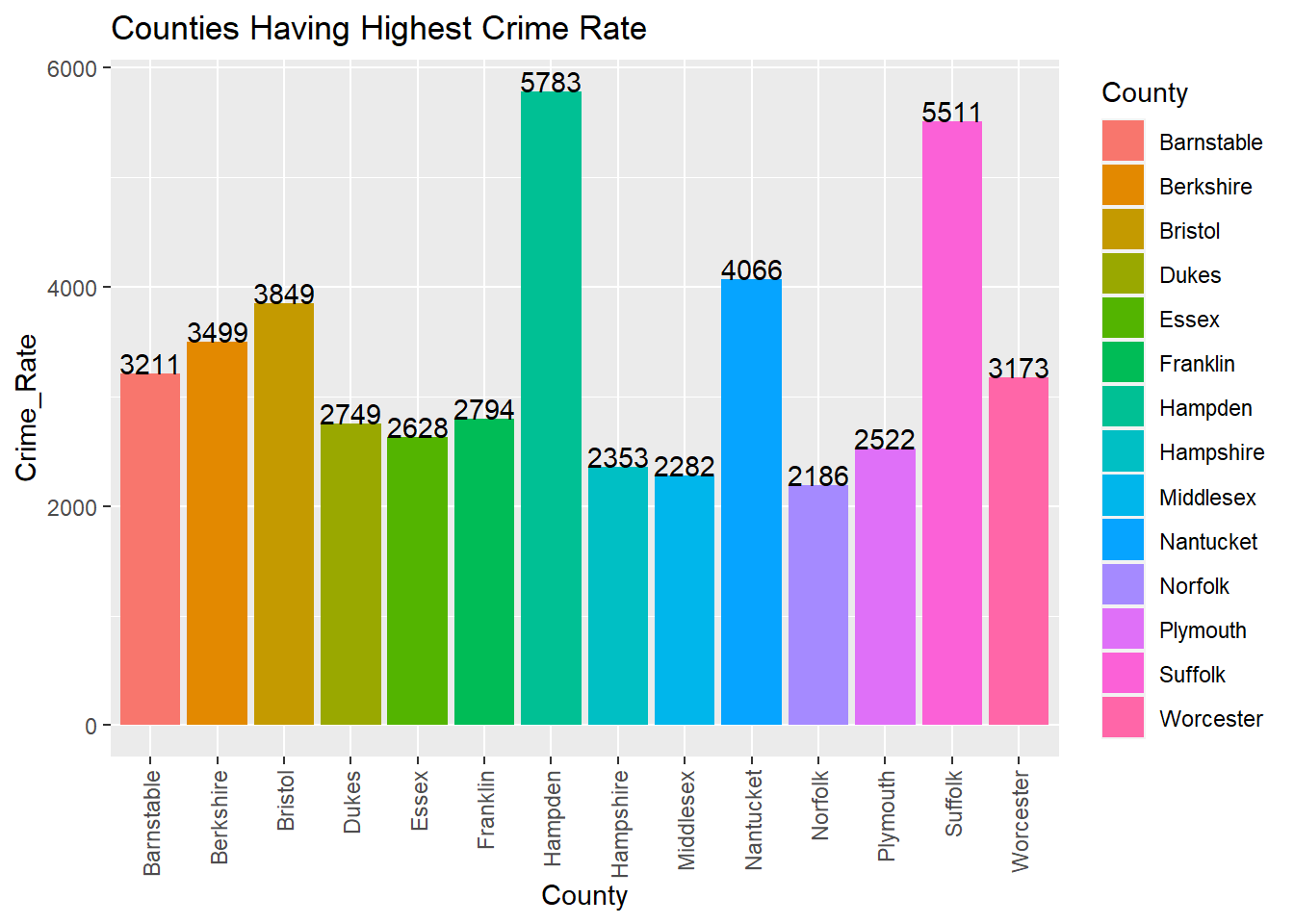
Finding which time of the day has the highest crime rate
Since the data had time of the day as a variable, I was curious to know what time of the day has more probability for a crime to happen. It was surprising to me to find out that 12pm-3pm had the most number of crimes followed by 3pm-6pm and 9am-12-pm. It is an interesting finding that nights are safer in Massachusetts than daytime as far as the number of crimes are concerned.
time_graph <- County_crime_total %>%
  pivot_longer(cols = (ends_with("am") | ends_with("pm")) | ends_with("noon"),
               names_to = "Time", values_to = "Crimes")
time_graph$Time<- factor(time_graph$Time,                 # Relevel group factor
                         levels = c("12am-3am", "3am-6am", "6am-9am", "9am-12pm", "12pm-3pm", "3pm-6pm", "6pm-9pm","9pm-12am"))

time_graph <- time_graph%>%
  group_by(Time) %>%
  summarise(Crimes = sum(Crimes))

time_graph %>%
  tail(10) %>%

  ggplot(aes(x = Time, y = Crimes)) +
  geom_point(shape = 21, color = "black", fill = "red", size = 4) +
  geom_line(color = "grey") +
  theme_ipsum() +
  ggtitle("Time When Most Crimes Happen") +
  theme(axis.text.x = element_text(angle = 90, vjust = 0.5, hjust=1))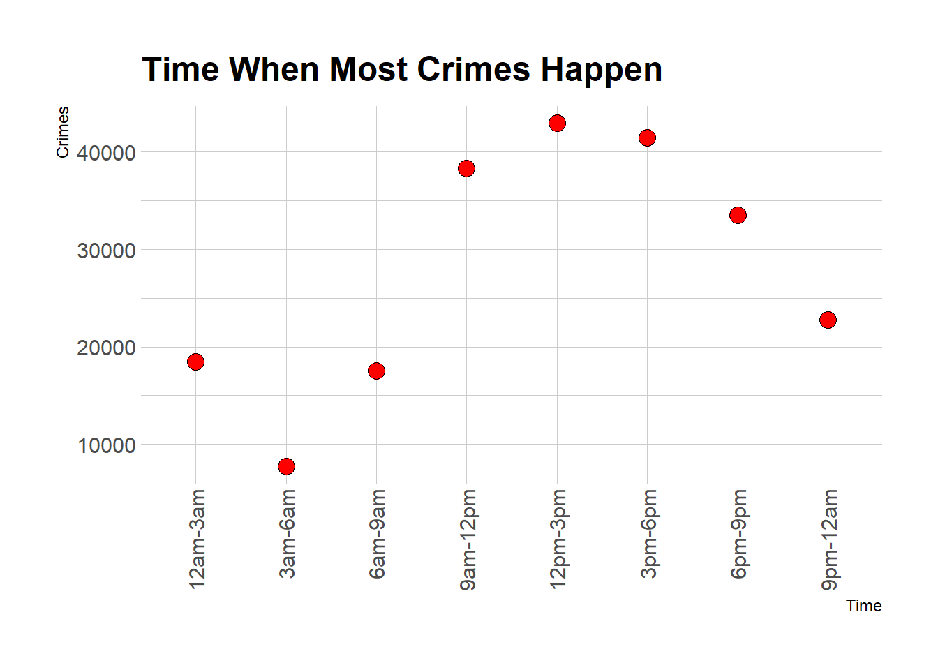
The counties having the most crime rate follow the same pattern in the time of the day in which more crimes happen.
df_crime_rate %>%
  filter(County == "Hampden" | County == "Suffolk"| County ==  "Nantucket") %>%
  group_by(County, Time) %>%
  summarise(CrimeRate = sum(Crime_Rate)) %>%
  ggplot(aes(x = County, y = CrimeRate, fill = Time)) +
    geom_bar(stat = "identity", position = position_dodge(0.9)) + theme(axis.text.x = element_text(angle = 90, vjust = 0.5, hjust=1)) +
  ggtitle("Time vs Counties with Top Crime Rates")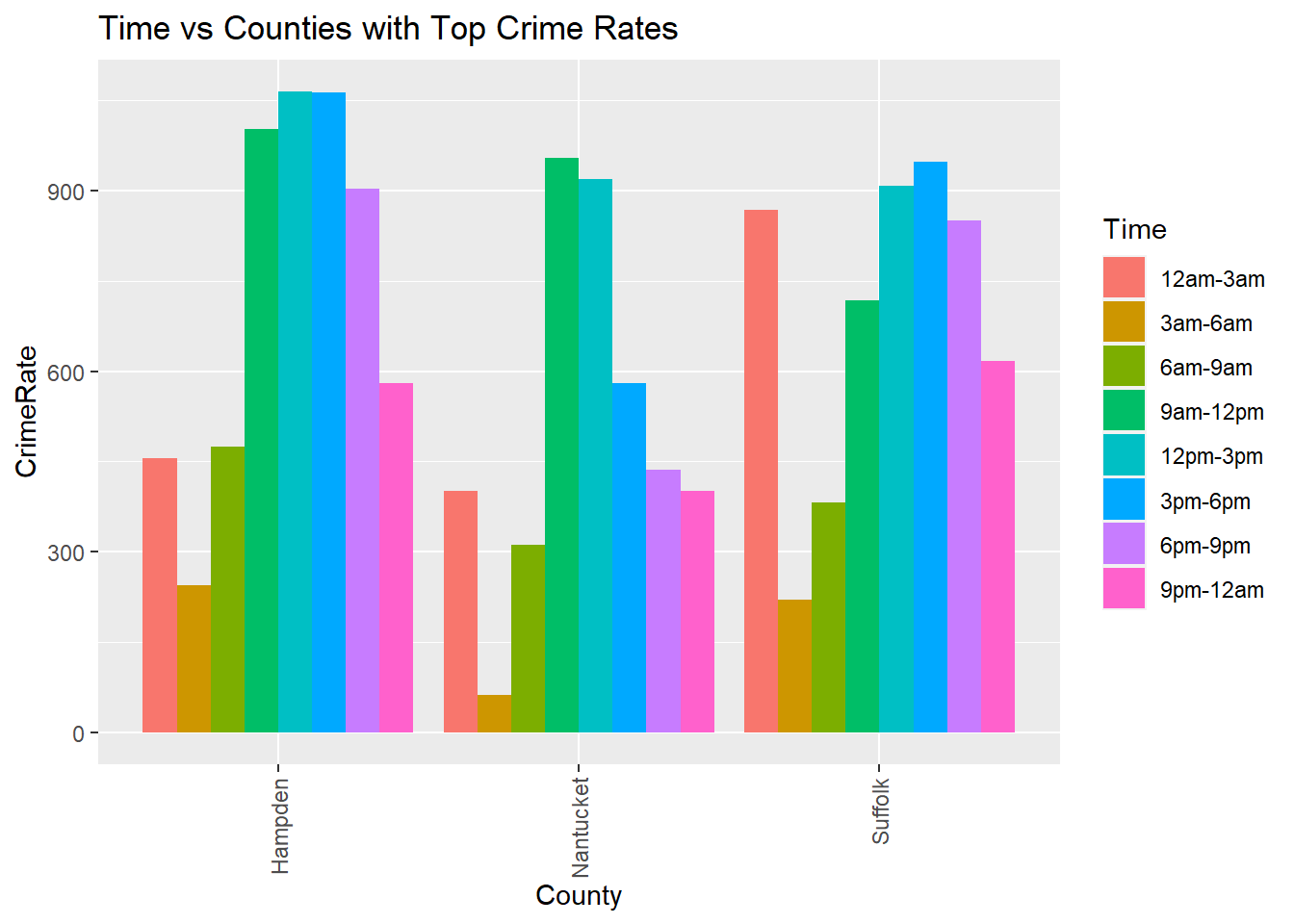
Analysing the reasons behind the crime rate.
# crimerate_reasons %>%
#   select(!income_factor)
As expected, Hampden (14.3%) and Suffolk (16.5%) had a higher rate of poverty but surprisingly, Nantucket has the lowest poverty rate (5.3%) even though Nantucket is in the top three counties in crime rate. However, Nantucket had the highest unemployment rate (11.1%) followed by Hampden (11.0%). Suffolk too had a comparatively higher unemployment rate (10.3%). When it comes to the percentage of young males of age 18-29, Hampshire is the top county regardless of its lower crime rate. But Suffolk and Hampden has some correlation between the crime rate and the percentage of young male. Hampden and Suffolk are having their median household income at $61600 and $85221 respectively which are lower than that of median household income of the Massachusetts state($89,026).
crimerate_reasons %>%
  pivot_longer(!County, names_to = "Reason", values_to = "Percent") %>%
  ggplot(aes(x=County, y=Percent, group=Reason, color=Reason)) +
  geom_line() +
  theme(axis.text.x = element_text(angle = 90, vjust = 0.5, hjust=1 )) +
  ggtitle("Causes of Increased Crime Rate")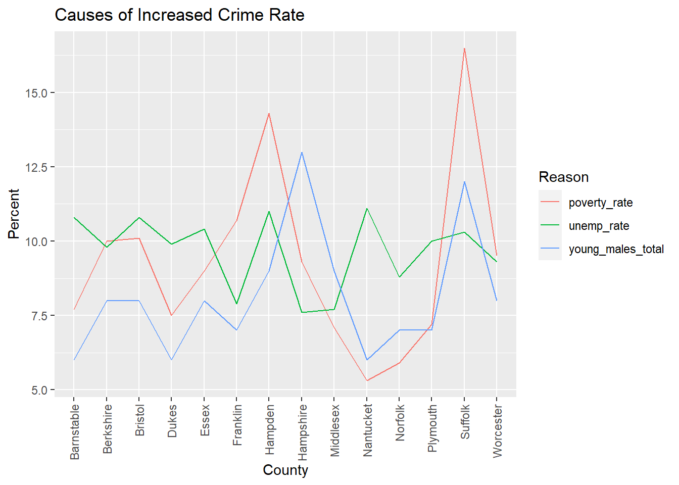
medianhh %>%
  ggplot(aes(x = County, y = median_hh_income, fill = median_hh_income)) +
    geom_bar(stat = "identity", position = position_dodge(0.9)) + theme(axis.text.x = element_text(angle = 90, vjust = 0.5, hjust=1)) +
  geom_text(aes(label = median_hh_income), vjust = 0, size = 3) +
  ggtitle("Countywise Median Household Income")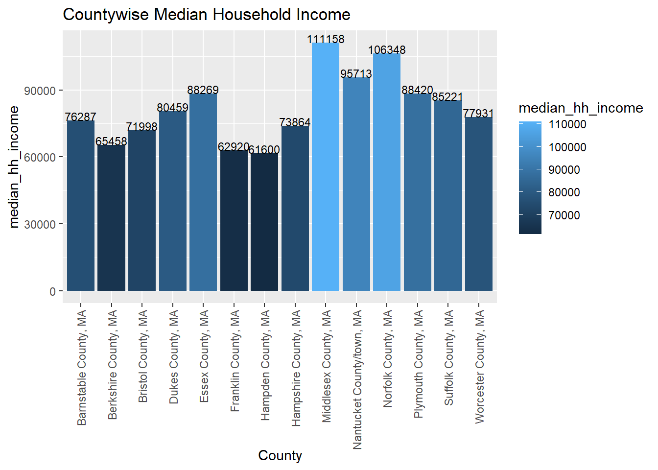
Conclusion
As expected, poverty, unemployment and median household income are showing some significant correlation with the crime rates in the counties of Massachusetts. Age and gender are moderating the other reasons to increase the crime rate.
Limitation of study and future scope
The study was done only with the data of 2021 and there are other factors that affect the crime rate. Due to the time constraint and unavailability of data, I am concluding my analysis here. But this analysis can be done in future with data of more years and including other variables that affect the crime rate.
Bibliography
Source of data:
1, https://masscrime.chs.state.ma.us/public/View/dispview.aspx
2, https://lmi.dua.eol.mass.gov/LMI/LaborForceAndUnemployment
3, https://data.census.gov
Programming Language: R
Course book : R for Data Science by Hadley Wickham & Garrett Grolemund