Code
library(tidyverse)
load("KarlaBarrett_Final.RData")

knitr::opts_chunk$set(echo = TRUE)Karla Barrett-Dexter
December 17, 2022
Maine is one of the top 10 least diverse states in the United States, although, it has seen an increase in immigrant and refugee resettlement rates over the past decade. This is something I consider quite a bit, as I manage a medical residency program and one of our goals is to increase the diversity of our faculty and residents to better reflect the demographics of the patient population we are caring for. This goal has yet to be achieved, so I thought it would be interesting to explore some data about migration patterns to and from Maine and ask, “is Maine becoming a more diverse state?”. This was the original impetus for my final paper, however, I also found it interesting to explore where people are moving to when they leave Maine and where they are moving from when they come to Maine.
The data chosen for this project details migration patterns for people born between the years 1984 and 1992. The data was captured by US Census, tax and HUD reporting.The primary variables of interest are: origin city/state (where the person was living at age 16) and destination city/state (where the person was living at age 26), race, and parental income level. The data was downloaded from migrationpatterns.org, a collaborative research project between the U.S. Census Bureau and Harvard University.
I tidied the data in a few ways:
After the initial tidying, I started zeroing in on the data for Maine, by creating new data frames for:
Some of the questions I wanted to explore at this point were:
To help me answer some of my questions, I did some setup by summarizing and joining of data such as migration patterns by Maine cities, states, race, and parental income. This setup was to aid in additional transformations and visualizations. A lot of this work ended up being unnecessary, but it was good practice!
Interestingly, there are only four Maine cities reflected in the data set: Portland, Bangor, Presque Isle, and Calais, which certainly turned my focus away from spending too much time looking into where exactly in Maine people moved to and from as those four cities do not paint a full picture. Portland is by far the largest city by population so it would not be surprising to see the most migration in and out of Portland due to that fact alone. The four cities included in the original data set as they are vastly different, especially Presque Isle and Calais, are two of the most remote towns in the state.
#Changed column names for ease of understanding
MillenialMigration <- MillenialMigration %>%
rename(Origin_Zone = o_cz,
Origin_City = o_cz_name,
Origin_State = o_state_name,
Dest_Zone = d_cz,
Dest_City = d_cz_name,
Dest_State = d_state_name,
Num_Migrators = n,
N_from_Origin = n_tot_o,
N_from_Dest = n_tot_d,
Race_ParentalIncome = pool,
Num_Migrators = n)Error in `rename()`:
! Can't rename columns that don't exist.
✖ Column `o_cz` doesn't exist.#I wanted to separate the Race and Parental Income data, in order to analyze the data separately in future iterations. I could not figure out a way to separate the two without putting a character in between. I used the following code to update the Race_ParentalIncome column to have an underscore in it. This was probably not the most efficient way to accomplish this outcome and it took me quite a while to get the code right.In addition, I found it was taking a very long time to run this code every time I returned to work on the assignment, so I decided to export the new CSV file and am writing in all the code used to get to this step as comments to show my work and continuing with the new file to avoid the time issues I was having running the code.
#MillenialMigration_ <- MillenialMigration %>%
# mutate(Race_ParentalIncome = stringr::str_replace(Race_ParentalIncome, "AsianQ1", "Asian_Q1"))%>%
# mutate(Race_ParentalIncome = stringr::str_replace(Race_ParentalIncome, "AsianQ2", "Asian_Q2"))%>%
# mutate(Race_ParentalIncome = stringr::str_replace(Race_ParentalIncome, "AsianQ3", "Asian_Q3"))%>%
# mutate(Race_ParentalIncome = stringr::str_replace(Race_ParentalIncome, "AsianQ4", "Asian_Q4"))%>%
# mutate(Race_ParentalIncome = stringr::str_replace(Race_ParentalIncome, "AsianQ5", "Asian_Q5"))%>%
# mutate(Race_ParentalIncome = stringr::str_replace(Race_ParentalIncome, "BlackQ1", "Black_Q1"))%>%
# mutate(Race_ParentalIncome = stringr::str_replace(Race_ParentalIncome, "BlackQ2", "Black_Q2"))%>%
# mutate(Race_ParentalIncome = stringr::str_replace(Race_ParentalIncome, "BlackQ3", "Black_Q3"))%>%
# mutate(Race_ParentalIncome = stringr::str_replace(Race_ParentalIncome, "BlackQ4", "Black_Q4"))%>%
# mutate(Race_ParentalIncome = stringr::str_replace(Race_ParentalIncome, "BlackQ5", "Black_Q5"))%>%
# mutate(Race_ParentalIncome = stringr::str_replace(Race_ParentalIncome, "HispanicQ1", "Hispanic_Q1"))%>%
# mutate(Race_ParentalIncome = stringr::str_replace(Race_ParentalIncome, "HispanicQ2", "Hispanic_Q2"))%>%
# mutate(Race_ParentalIncome = stringr::str_replace(Race_ParentalIncome, "HispanicQ3", "Hispanic_Q3"))%>%
# mutate(Race_ParentalIncome = stringr::str_replace(Race_ParentalIncome, "HispanicQ4", "Hispanic_Q4"))%>%
# mutate(Race_ParentalIncome = stringr::str_replace(Race_ParentalIncome, "HispanicQ5", "Hispanic_Q5"))%>%
# mutate(Race_ParentalIncome = stringr::str_replace(Race_ParentalIncome, "OtherQ1", "Other_Q1"))%>%
# mutate(Race_ParentalIncome = stringr::str_replace(Race_ParentalIncome, "OtherQ2", "Other_Q2"))%>%
# mutate(Race_ParentalIncome = stringr::str_replace(Race_ParentalIncome, "OtherQ3", "Other_Q3"))%>%
# mutate(Race_ParentalIncome = stringr::str_replace(Race_ParentalIncome, "OtherQ4", "Other_Q4"))%>%
# mutate(Race_ParentalIncome = stringr::str_replace(Race_ParentalIncome, "OtherQ5", "Other_Q5"))%>%
# mutate(Race_ParentalIncome = stringr::str_replace(Race_ParentalIncome, "WhiteQ1", "White_Q1"))%>%
# mutate(Race_ParentalIncome = stringr::str_replace(Race_ParentalIncome, "WhiteQ2", "White_Q2"))%>%
# mutate(Race_ParentalIncome = stringr::str_replace(Race_ParentalIncome, "WhiteQ3", "White_Q3"))%>%
# mutate(Race_ParentalIncome = stringr::str_replace(Race_ParentalIncome, "WhiteQ4", "White_Q4"))%>%
# mutate(Race_ParentalIncome = stringr::str_replace(Race_ParentalIncome, "WhiteQ5", "White_Q5"))
#I used the following code to check my work
#MigratorsByRace_Income <- MillenialMigration_ %>%
# group_by(Race_ParentalIncome) %>%
#summarise(Freq = sum(Num_Migrators))
#print(n=30, MigratorsByRace_Income)
#The following code was used to separate the column and create two new columns, one for Race and one for Parental Income.
#MillenialMigration_Sep <- separate(MillenialMigration_, Race_ParentalIncome, into = c("Race", "Parental_Income"), sep = "_")
#MillenialMigration_Sep
#The following code was used to create a new CSV file with the separated columns.
#write.csv(MillenialMigration_Sep, file = "C:\\Users\\kbarr\\OneDrive\\Documents\\GitHub\\601_Fall_2022\\posts\\MillenialMigration_Sep.csv", row.names = FALSE)
#Read in updated data set with separate columns for race and parental income
# MillenialMigration_Sep <- read_csv("_data/MillenialMigration_Sep.csv")
head(MillenialMigration_Sep) [1] "Origin_Zone" "Origin_City" "Origin_State" "Dest_Zone"
[5] "Dest_City" "Dest_State" "Num_Migrators" "N_from_Origin"
[9] "N_from_Dest" "Race" "Parental_Income" "pr_d_o"
[13] "pr_o_d" #The following code was used to set up smaller data frames to aid in visualizations and analysis
#Filter for Maine as destination state
MillenialMigration_to_Maine <- MillenialMigration_Sep %>%
filter(Dest_State== "Maine")
#Filter for Maine as origin state
MillenialMigration_from_Maine <- MillenialMigration_Sep %>%
filter(Origin_State== "Maine")
#Summarise total migrators to cities in Maine
MillenialMigration_to_Maine_Sum <- MillenialMigration_to_Maine %>%
group_by(Dest_City) %>%
summarise(Num_Migrators_to_Maine = sum(Num_Migrators))
#Rename City variable to prep for join
MillenialMigration_to_Maine_Sum <- MillenialMigration_to_Maine_Sum %>%
rename(City = Dest_City)
#Summarise total migrators from cities in Maine
MillenialMigration_from_Maine_Sum <- MillenialMigration_from_Maine %>%
group_by(Origin_City) %>%
summarise(Num_Migrators_from_Maine = sum(Num_Migrators))
#Rename City variable to prep for join
MillenialMigration_from_Maine_Sum <- MillenialMigration_from_Maine_Sum %>%
rename(City = Origin_City)
#Join totals to and from Maine
Migration_In_And_Out_Maine <- inner_join(MillenialMigration_from_Maine_Sum, MillenialMigration_to_Maine_Sum, by="City")
Migration_In_And_Out_Maine#Migrators by race/income - all data
MigratorsByIncome <- MillenialMigration_Sep %>%
group_by(Parental_Income) %>%
summarise(Num_Migrators= sum(Num_Migrators))
MigratorsByRace <- MillenialMigration_Sep %>%
group_by(Race) %>%
summarise(Num_Migrators= sum(Num_Migrators))
#Migrators by race/income - Maine data
Migration_to_Maine_Race <- MillenialMigration_to_Maine %>%
group_by(Race) %>%
summarise(Num_Migrators= sum(Num_Migrators))
Migration_to_Maine_Income <- MillenialMigration_to_Maine %>%
group_by(Parental_Income) %>%
summarise(Num_Migrators= sum(Num_Migrators))
Migration_from_Maine_Race <- MillenialMigration_to_Maine %>%
group_by(Race) %>%
summarise(Num_Migrators= sum(Num_Migrators))
Migration_from_Maine_Income <- MillenialMigration_to_Maine %>%
group_by(Parental_Income) %>%
summarise(Num_Migrators= sum(Num_Migrators))
# Tidy to Maine by State
To_Maine_Sum_By_State <- MillenialMigration_to_Maine %>%
group_by(Origin_State) %>%
summarise(Num_Migrators = sum(Num_Migrators))
To_Maine_Sum_By_State <- To_Maine_Sum_By_State %>% arrange(desc(Num_Migrators))
To_Maine_Sum_By_State <- To_Maine_Sum_By_State %>%
rename(Num_Migrators_to_Maine = Num_Migrators)
To_Maine_Sum_By_State <- To_Maine_Sum_By_State %>%
rename(State = Origin_State)
# Tidy from Maine by State
From_Maine_Sum_By_State <- MillenialMigration_from_Maine %>%
group_by(Dest_State) %>%
summarise(Num_Migrators = sum(Num_Migrators))
From_Maine_Sum_By_State <- From_Maine_Sum_By_State %>% arrange(desc(Num_Migrators))
From_Maine_Sum_By_State <- From_Maine_Sum_By_State %>%
rename(Num_Migrators_from_Maine = Num_Migrators)
From_Maine_Sum_By_State <- From_Maine_Sum_By_State %>%
rename(State = Dest_State)
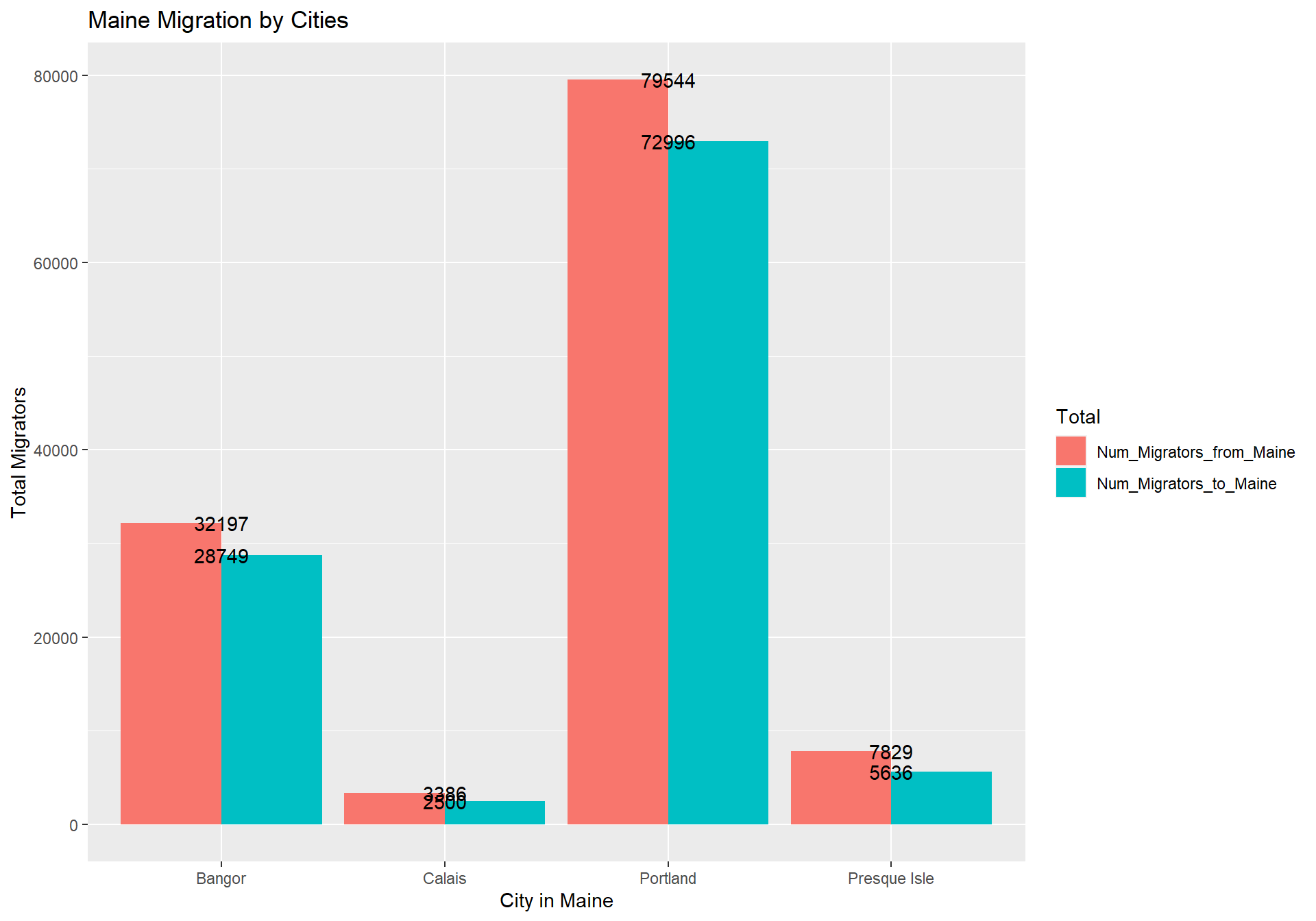
To_Maine_Sum_By_StateThe first visualization I created was simply to compare the total number of migrators in and out of each city.Portland and Bangor saw the most migration, Calais and Presque Isle saw the least, the results were not surprising given the population size of each city as mentioned before. Each city experienced more migration out than in.
The next question I explored was where are people migrating to Maine from? It turns out, the vast most of the migration in Maine is occurring within Maine. After inter-state movement, the largest group of people to move to Maine were from other Northeastern states (VT, NY, CT, NH, etc.). I originally made the visualization to include all states, but decided to filter it down to the top 10. I also chose to put the states on the y axis for a better visual representation.
#| label: Where did they come from?
#| warning: false
#Original code for plot with all states: ggplot(To_Maine_Sum_By_State, aes(Num_Migrators_to_Maine, State)) + geom_bar(stat = "identity", fill = "cadetblue")
To_Maine_Sum_By_State %>%
filter(Num_Migrators_to_Maine >= 637) %>%
ggplot(aes(Num_Migrators_to_Maine, State)) + geom_bar(stat = "identity", fill = "cadetblue") + labs(title = "Where Did People Come to Maine From?", x = "Number of Migrators")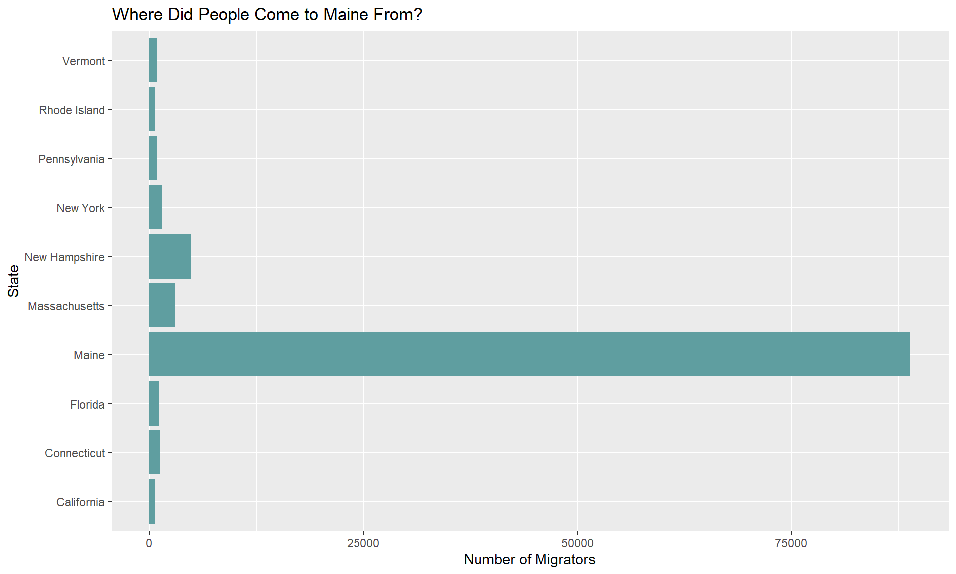
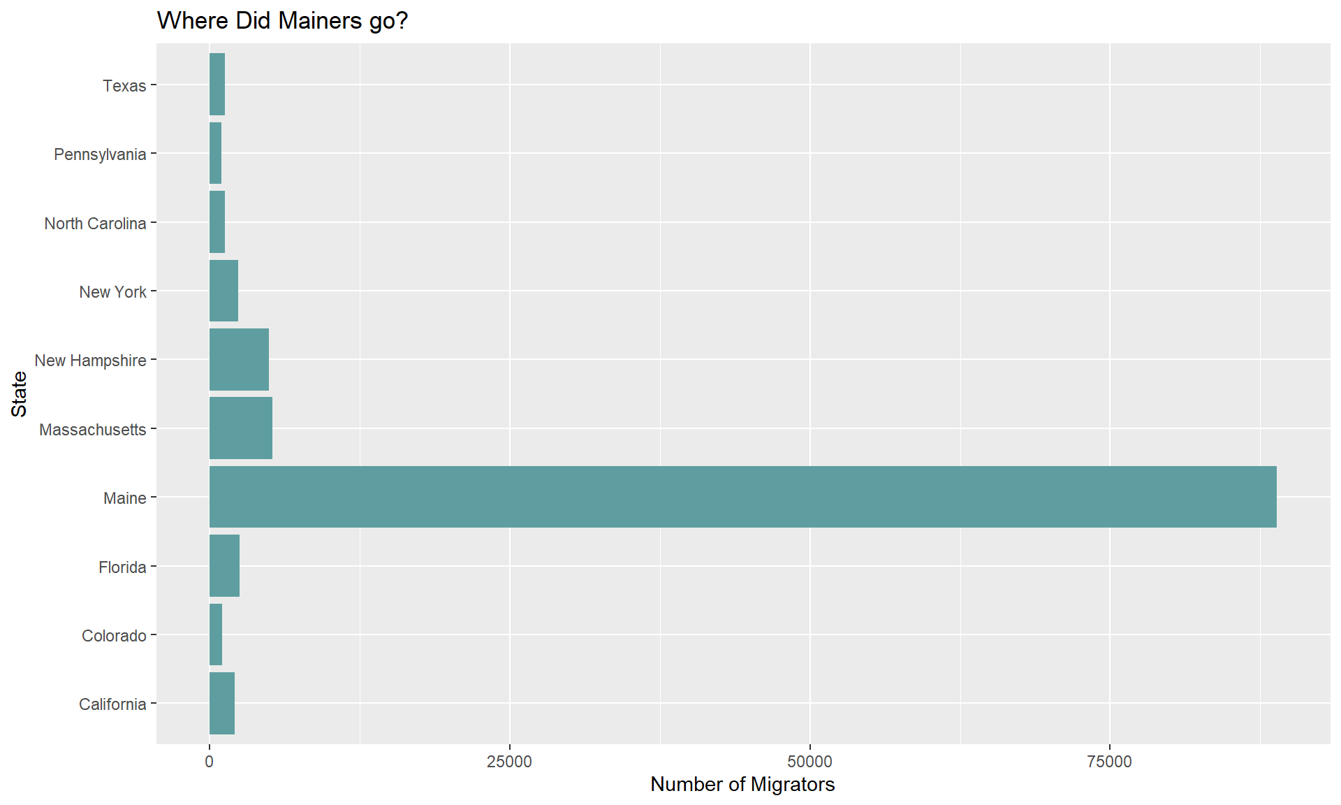
After, I used the same process to create a graph showing where people from Maine were moving to. Seven of the top 10 states showed up on both lists. The three states on the list of places people moved to Maine from but not on the list of states people moved to were: Vermont, Rhode Island, and Connecticut. Alternatively, the three states not in the top ten list for states people moved from are: Texas, North Carolina, and Colorado. Anecdotally, I am not surprised to see Colorado in the top ten list of states Mainers move to, skiers love to go out west!
Finally, I wanted to see the movement in and out of each state on the same graph. I created two versions of this, the second with a facet wrap after creating a new column with grouped values.The facet wrap helped spread the plot points out and I believe made it a better visual aid. Although, there is not much to take away from these charts other than viewing the difference between migration to and from Maine between different states.
# Join to and from Maine
To_and_From_Maine_ByState <- inner_join(To_Maine_Sum_By_State, From_Maine_Sum_By_State, by="State")
To_and_From_Maine_ByState_Combined <- To_and_From_Maine_ByState %>% gather(Total, Value, -State)
ggplot(To_and_From_Maine_ByState_Combined, aes(x = Value, y = State)) +
geom_point() + labs(title = "Where Did People Move to and From", y = "State", x = "Value")+
geom_point(aes(color = factor(Total)))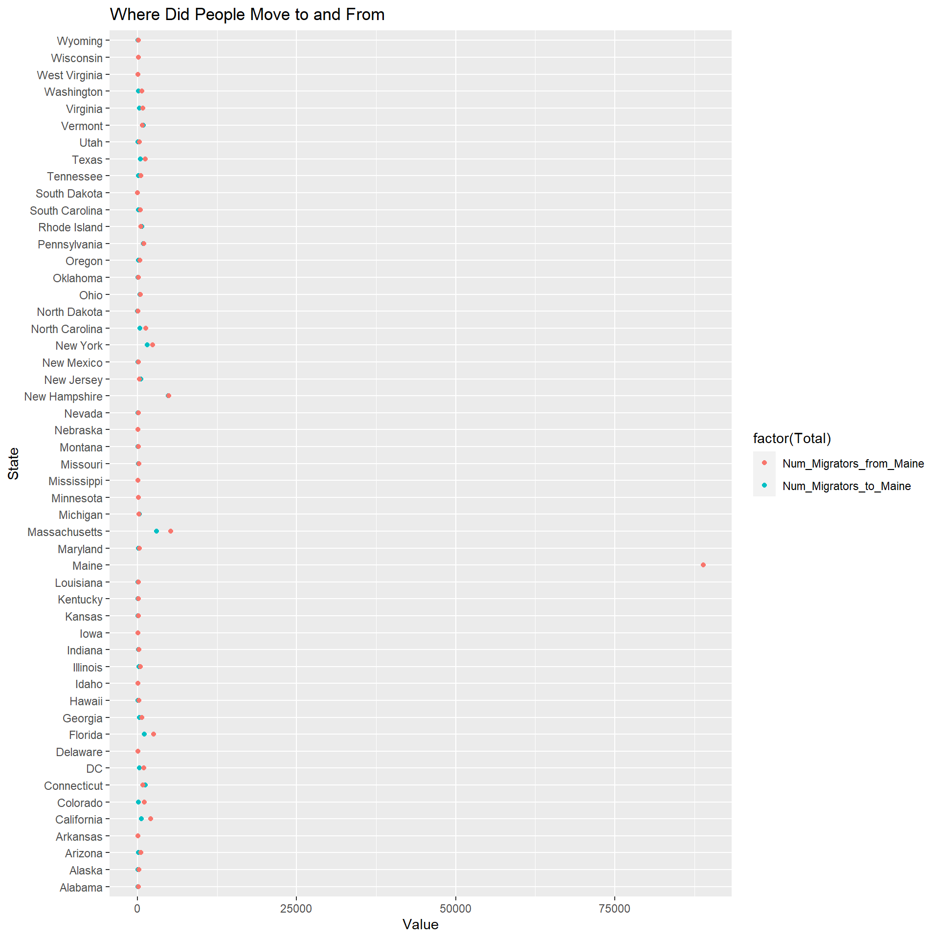
ToAndFrom <- To_and_From_Maine_ByState_Combined %>% mutate(Total = case_when(Value <100 ~ "Under 100 Migrators",
Value <500 ~ "Under 500 Migrators",
Value >501 ~ "Over 500 Migrators"))
ToAndFrom <- To_and_From_Maine_ByState_Combined %>%
select(State, Total, Value)%>%
mutate(
Value_Groups = case_when(Value <100 ~ "Under 100 Migrators",
Value <500 ~ "Under 500 Migrators",
Value >501 ~ "Over 500 Migrators"))
ToAndFrom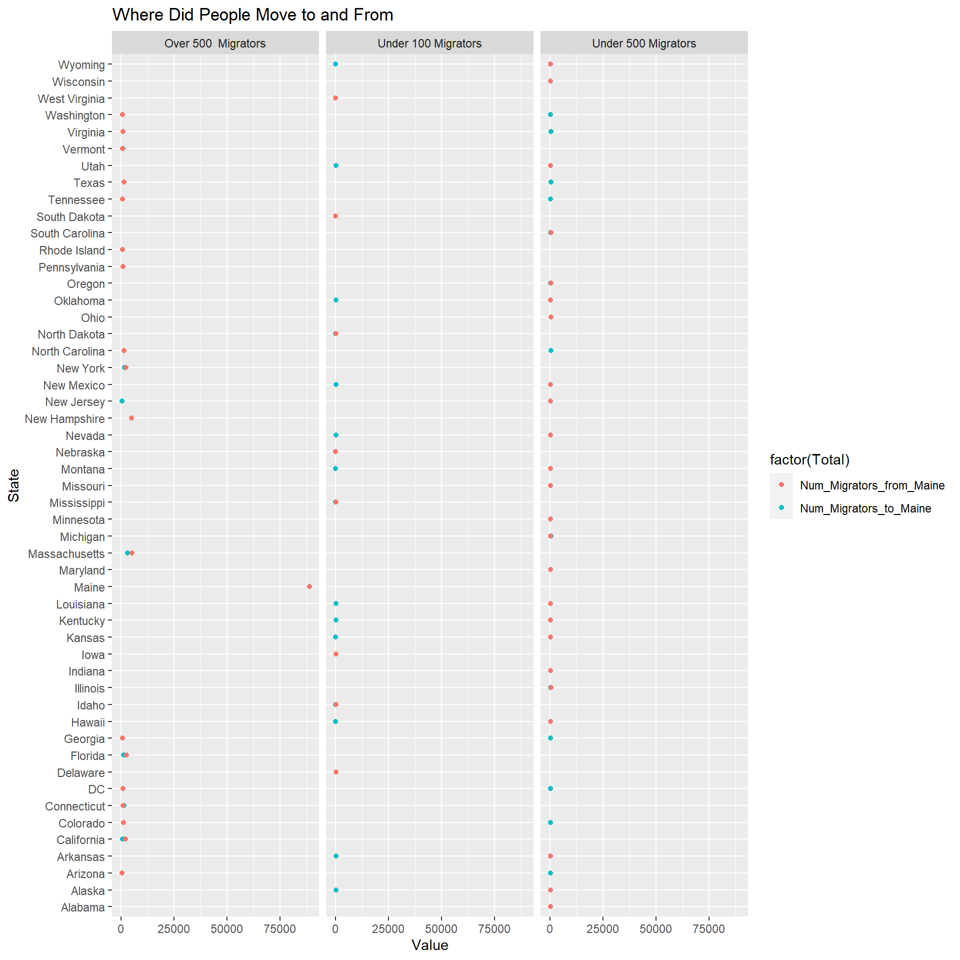
I moved on to exploring the relationship between migration patterns and race and income levels (specifically parental income levels, which I think is important to note as generational wealth is a significant factor in someone’s ability to move).
I grouped the data by parental income or race for both Maine data, and the original data set as a whole, then summarized the number of migrators in each category. I renamed columns in order to join the the Maine data and the total data in one data frame that would allow me to compare the data in the same visualization.
The migration patterns by race were similar for both Maine and the entire data set. The income category however saw an oddity, the highest parental income quintile in Maine saw very little migration compared to the migration patterns for the whole data set.
Given how much more migration is seen among white populations, I wanted to focus in on non-white populations to help answer my question of “is Maine becoming more diverse”. I found the difference between the number of non-white migrators that came to Maine and left Maine and created a bar chart. There was a very slight increase in black and hispanic populations, but asian and “other” both dropped. Overall, based on this limited data set, it appears Maine is not becoming more diverse.
#Migrators by Income Data Transformation
MigratorsByIncome <- MillenialMigration_Sep %>%
group_by(Parental_Income) %>%
summarise(Num_Migrators= sum(Num_Migrators)) %>%
rename(Num_All_Income = Num_Migrators)
Maine_Migration_Income <- MillenialMigration_Maine_All %>%
group_by(Parental_Income) %>%
summarise(Num_Migrators= sum(Num_Migrators)) %>%
rename(Num_Maine_Income = Num_Migrators)
Maine_vs_All_Income <- inner_join(MigratorsByIncome, Maine_Migration_Income, by="Parental_Income")
Maine_vs_All_Income_Transform <- Maine_vs_All_Income %>% gather(AllOrMaine, Num_Migrators, -Parental_Income)
Maine_vs_All_Income_Transform_Groups<- Maine_vs_All_Income_Transform %>%
select(Parental_Income, Num_Migrators, AllOrMaine)%>%
mutate(
AllorMaineGroups = case_when(AllOrMaine == "Num_All_Income" ~ "All Data", AllOrMaine == "Num_Maine_Income" ~ "Maine Data"))
ggplot(Maine_vs_All_Income_Transform_Groups, aes(x = Num_Migrators, y = Parental_Income)) +
geom_count()+ labs(title = "Migration by Income Level - Maine vs All Data")+
geom_count(aes(color = factor(Parental_Income)))+
facet_wrap(~AllorMaineGroups, scales = "free")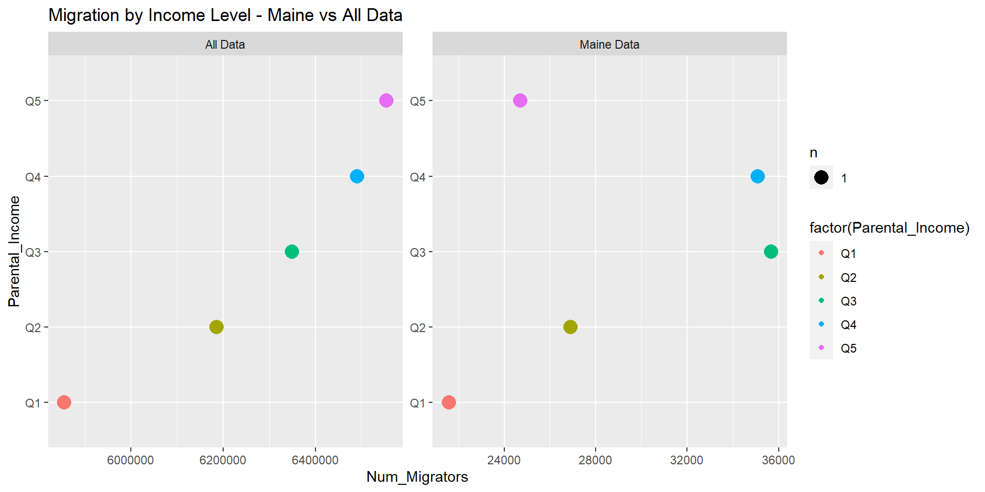
#Migrators by Race Data Transformation
MigratorsByRace <- MillenialMigration_Sep %>%
group_by(Race) %>%
summarise(Num_Migrators= sum(Num_Migrators)) %>%
rename(Num_All_Race = Num_Migrators)
Maine_Migration_Race <- MillenialMigration_Maine_All %>%
group_by(Race) %>%
summarise(Num_Migrators= sum(Num_Migrators)) %>%
rename(Num_Maine_Race = Num_Migrators)
Maine_vs_All_Race <- inner_join(MigratorsByRace, Maine_Migration_Race, by="Race")
Maine_vs_All_Race_Transform <- Maine_vs_All_Race %>% gather(AllOrMaine, Num_Migrators, -Race)
Maine_vs_All_Race_Transform_Groups<- Maine_vs_All_Race_Transform %>%
select(Race, Num_Migrators, AllOrMaine)%>%
mutate(
AllorMaineGroups = case_when(AllOrMaine == "Num_All_Race" ~ "All Data", AllOrMaine == "Num_Maine_Race" ~ "Maine Data"))
ggplot(Maine_vs_All_Race_Transform_Groups, aes(x = Num_Migrators, y = Race)) +
geom_count()+ labs(title = "Migration by Race - Maine vs All Data")+
geom_count(aes(color = factor(AllorMaineGroups)))+
scale_color_manual(values = c("All Data" = "thistle4", "Maine Data" = "cadetblue"))+
facet_wrap(~AllorMaineGroups, scales = "free")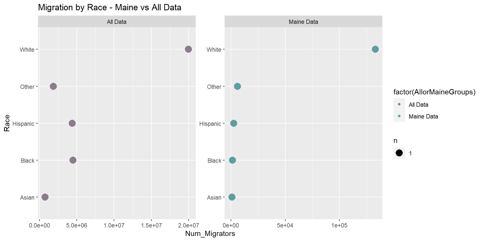
#Exploring non-white migration to and from Maine
To_Maine_nonWhite_Migration <-MillenialMigration_to_Maine%>%
filter(Race != "White")%>%
group_by(Race) %>%
summarise(Num_Migrators= sum(Num_Migrators)) %>%
rename(Num_to_Maine_Race = Num_Migrators)
From_Maine_nonWhite_Migration <- MillenialMigration_from_Maine%>%
filter(Race != "White")%>%
group_by(Race) %>%
summarise(Num_Migrators= sum(Num_Migrators)) %>%
rename(Num_from_Maine_Race = Num_Migrators)
Maine_non_white_migration <- inner_join(To_Maine_nonWhite_Migration, From_Maine_nonWhite_Migration, by="Race")
Maine_non_white_migration_difference <- Maine_non_white_migration%>%
select(Race, Num_from_Maine_Race, Num_to_Maine_Race) %>%
mutate(Difference = Num_to_Maine_Race - Num_from_Maine_Race)
Maine_non_white_migration_difference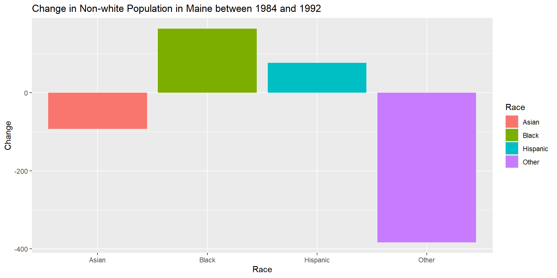
I did not read the full report available on migrationpatterns.org until after I finished my project, as I wanted to avoid the analysis of much more experienced researchers affecting my approach to the project, both the questions I wanted to investigate and the scope of my abilities. For example, after working with the data, I determined the best visualizations to use would be bar charts and point plots, due to the fact that I was only working with one numerical variable. Upon reviewing the report, I discovered there are so many more possibilities and I am both glad I did not see it beforehand (to keep my goal output realistic) and a bit disappointed I did not experiment more with histograms box plots, for example. Also, after reviewing the report, I would like to learn how to plot the migration data on a map of the U.S. I researched how to do it a bit and determined it was not feasible for this project but I would like to keep trying in the future.
One of the most challenging aspects of this project was the time spent trying to find tiny little mistakes that affected large portions of my work (a missed comma, using the wrong column name, using + when I needed to use %>%), but ultimately, I found the experience to be incredibly valuable as I am now much better at spotting mistakes and every problem solved, no matter how little felt like a huge win. Another challenge I had that I did not end up solving is changing the order of the facets in my charts. I searched for multiple hours for a solution to no avail and the order of the facets did not end up in ascending or descending order.
One of the questions I was looking to answer with this project was, “is Maine becoming more diverse?”. The conclusion I came to with this data set is, no. However, there are a number of factors that limited my ability to fully explore this question:
Other questions I still have are:
Textbook: Grolemund, G., & Wickham, H. (2017). R for Data Science. O’Reilly Media.
Data source: U.S Census Bureau, Harvard University. (n.d.). Young Adult Migration. Migration Patterns. Retrieved December 18, 2022, from https://migrationpatterns.org/
R: R Core Team (2022). R: A language and environment for statistical computing. R Foundation for Statistical Computing, Vienna, Austria. URL https://www.R-project.org/.
Wickham H (2016). ggplot2: Elegant Graphics for Data Analysis. Springer-Verlag New York. ISBN 978-3-319-24277-4, https://ggplot2.tidyverse.org.
Sape Research Group. (n.d.) ggplot2 Quick Reference: colour (and fill). Software and programmer Efficiency Research Group. Retrieved December 18, 2022, from http://sape.inf.usi.ch/quick-reference/ggplot2/colour
https://datatofish.com/export-dataframe-to-csv-in-r/
Data to Fish. (n.d.). How to Export DataFrame to CSV in R. Retrieved December 18, 2022, fromdatatofish.com/export-dataframe-to-csv-in-r/
:::
---
title: "Final Project"
author: "Karla Barrett-Dexter"
desription: "Millenial Migration"
date: "12/17/2022"
format:
html:
toc: true
code-fold: true
code-copy: true
code-tools: true
df-print: paged
categories:
- Final Project
- Karla Barrett-Dexter
---
```{r}
#| label: setup
#| warning: false
library(tidyverse)
load("KarlaBarrett_Final.RData")
knitr::opts_chunk$set(echo = TRUE)
```
## Introduction
Maine is one of the top 10 least diverse states in the United States, although, it has seen an increase in immigrant and refugee resettlement rates over the past decade. This is something I consider quite a bit, as I manage a medical residency program and one of our goals is to increase the diversity of our faculty and residents to better reflect the demographics of the patient population we are caring for. This goal has yet to be achieved, so I thought it would be interesting to explore some data about migration patterns to and from Maine and ask, "is Maine becoming a more diverse state?". This was the original impetus for my final paper, however, I also found it interesting to explore where people are moving to when they leave Maine and where they are moving from when they come to Maine.
## Data
The data chosen for this project details migration patterns for people born between the years 1984 and 1992. The data was captured by US Census, tax and HUD reporting.The primary variables of interest are: origin city/state (where the person was living at age 16) and destination city/state (where the person was living at age 26), race, and parental income level. The data was downloaded from migrationpatterns.org, a collaborative research project between the U.S. Census Bureau and Harvard University.
I tidied the data in a few ways:
1. Read in the data and labeled the original data frame "MillenialMigration"
2. Renamed the column names for ease of understanding (e.g. d_cz_name became Dest_City)
3. The race and parental income data was combined in one column in the original data set. I decided to separate out the two data points into different columns by using the mutate function to replace the original character format (e.g. AsianQ1) to a format that included an underscore (e.g. Asian_Q1) so I could then use the separate function, with the underscore as the separator to create the two distinct columns.I thought it would be interesting to be able to explore the race and income level data points on their own.
4. Finally, after struggling with the lag time to process all the code to accomplish separating out the columns, I opted to save the new data frame as a csv file using write.csv so I could continue on with the project without waiting for the code to run from start to finish every time I revisited my work. I have included all the code used to get to this point as comments.
After the initial tidying, I started zeroing in on the data for Maine, by creating new data frames for:
1. Migration to Maine
2. Migration from Maine
3. Both migration to and from Maine
Some of the questions I wanted to explore at this point were:
1. Did more people migrate to or from Maine?
2. Migration to Maine
- Where did people migrate from?
- Where in Maine did they settle?
- Is there a clear race or parental income level pattern for migration into the state? Is there a difference between a popular urban location such as Portland, and a more rural city such as Augusta?
3. Migration from Maine
- Where did they go?
- Race or parental income level patterns?
To help me answer some of my questions, I did some setup by summarizing and joining of data such as migration patterns by Maine cities, states, race, and parental income. This setup was to aid in additional transformations and visualizations. A lot of this work ended up being unnecessary, but it was good practice!
Interestingly, there are only four Maine cities reflected in the data set: Portland, Bangor, Presque Isle, and Calais, which certainly turned my focus away from spending too much time looking into where exactly in Maine people moved to and from as those four cities do not paint a full picture. Portland is by far the largest city by population so it would not be surprising to see the most migration in and out of Portland due to that fact alone. The four cities included in the original data set as they are vastly different, especially Presque Isle and Calais, are two of the most remote towns in the state.
```{r}
#| label: Data Transformations
#| warning: false
#|
#Read in original data set
# MillenialMigration <- read_csv("_data/od.csv")
head(MillenialMigration)
#Changed column names for ease of understanding
MillenialMigration <- MillenialMigration %>%
  rename(Origin_Zone = o_cz,
         Origin_City = o_cz_name,
         Origin_State = o_state_name,
         Dest_Zone = d_cz,
         Dest_City = d_cz_name,
         Dest_State = d_state_name,
         Num_Migrators = n,
         N_from_Origin = n_tot_o,
         N_from_Dest = n_tot_d,
         Race_ParentalIncome = pool,
         Num_Migrators = n)
MillenialMigration
#I wanted to separate the Race and Parental Income data, in order to analyze the data separately in future iterations. I could not figure out a way to separate the two  without putting a character in between. I used the following code to update the Race_ParentalIncome column to have an underscore in it. This was probably  not the most efficient way to accomplish this outcome and it took me quite a while to get the code right.In addition, I found it was taking a very long time to run this code every time I returned to work on the assignment, so I decided to export the new CSV file and am writing in all the code used to get to this step as comments to show my work and continuing with the new file to avoid the time issues I was having running the code.
#MillenialMigration_ <- MillenialMigration %>%
 # mutate(Race_ParentalIncome = stringr::str_replace(Race_ParentalIncome, "AsianQ1", "Asian_Q1"))%>%
  # mutate(Race_ParentalIncome = stringr::str_replace(Race_ParentalIncome, "AsianQ2", "Asian_Q2"))%>%
 #  mutate(Race_ParentalIncome = stringr::str_replace(Race_ParentalIncome, "AsianQ3", "Asian_Q3"))%>%
 #  mutate(Race_ParentalIncome = stringr::str_replace(Race_ParentalIncome, "AsianQ4", "Asian_Q4"))%>%
 #  mutate(Race_ParentalIncome = stringr::str_replace(Race_ParentalIncome, "AsianQ5", "Asian_Q5"))%>%
 #  mutate(Race_ParentalIncome = stringr::str_replace(Race_ParentalIncome, "BlackQ1", "Black_Q1"))%>%
 #  mutate(Race_ParentalIncome = stringr::str_replace(Race_ParentalIncome, "BlackQ2", "Black_Q2"))%>%
 #  mutate(Race_ParentalIncome = stringr::str_replace(Race_ParentalIncome, "BlackQ3", "Black_Q3"))%>%
 #  mutate(Race_ParentalIncome = stringr::str_replace(Race_ParentalIncome, "BlackQ4", "Black_Q4"))%>%
 #  mutate(Race_ParentalIncome = stringr::str_replace(Race_ParentalIncome, "BlackQ5", "Black_Q5"))%>%
 #  mutate(Race_ParentalIncome = stringr::str_replace(Race_ParentalIncome, "HispanicQ1", "Hispanic_Q1"))%>%
 #  mutate(Race_ParentalIncome = stringr::str_replace(Race_ParentalIncome, "HispanicQ2", "Hispanic_Q2"))%>%
 #  mutate(Race_ParentalIncome = stringr::str_replace(Race_ParentalIncome, "HispanicQ3", "Hispanic_Q3"))%>%
 #  mutate(Race_ParentalIncome = stringr::str_replace(Race_ParentalIncome, "HispanicQ4", "Hispanic_Q4"))%>%
 # mutate(Race_ParentalIncome = stringr::str_replace(Race_ParentalIncome, "HispanicQ5", "Hispanic_Q5"))%>%
 # mutate(Race_ParentalIncome = stringr::str_replace(Race_ParentalIncome, "OtherQ1", "Other_Q1"))%>%
 # mutate(Race_ParentalIncome = stringr::str_replace(Race_ParentalIncome, "OtherQ2", "Other_Q2"))%>%
 # mutate(Race_ParentalIncome = stringr::str_replace(Race_ParentalIncome, "OtherQ3", "Other_Q3"))%>%
 # mutate(Race_ParentalIncome = stringr::str_replace(Race_ParentalIncome, "OtherQ4", "Other_Q4"))%>%
 # mutate(Race_ParentalIncome = stringr::str_replace(Race_ParentalIncome, "OtherQ5", "Other_Q5"))%>%
 # mutate(Race_ParentalIncome = stringr::str_replace(Race_ParentalIncome, "WhiteQ1", "White_Q1"))%>%
 # mutate(Race_ParentalIncome = stringr::str_replace(Race_ParentalIncome, "WhiteQ2", "White_Q2"))%>%
 # mutate(Race_ParentalIncome = stringr::str_replace(Race_ParentalIncome, "WhiteQ3", "White_Q3"))%>%
 # mutate(Race_ParentalIncome = stringr::str_replace(Race_ParentalIncome, "WhiteQ4", "White_Q4"))%>%
 #  mutate(Race_ParentalIncome = stringr::str_replace(Race_ParentalIncome, "WhiteQ5", "White_Q5"))

#I used the following code to check my work
#MigratorsByRace_Income <- MillenialMigration_ %>%
 # group_by(Race_ParentalIncome) %>%
  #summarise(Freq = sum(Num_Migrators))
#print(n=30, MigratorsByRace_Income)

#The following code was used to separate the column and create two new columns, one for Race and one for Parental Income.
#MillenialMigration_Sep <- separate(MillenialMigration_, Race_ParentalIncome, into = c("Race", "Parental_Income"), sep = "_")
#MillenialMigration_Sep

#The following code was used to create a new CSV file with the separated columns.
#write.csv(MillenialMigration_Sep, file = "C:\\Users\\kbarr\\OneDrive\\Documents\\GitHub\\601_Fall_2022\\posts\\MillenialMigration_Sep.csv", row.names = FALSE)

#Read in updated data set with separate columns for race and parental income
# MillenialMigration_Sep <- read_csv("_data/MillenialMigration_Sep.csv")
head(MillenialMigration_Sep)
# save.image("KarlaBarrett_Final.RData")
colnames(MillenialMigration_Sep)
#The following code was used to set up smaller data frames to aid in visualizations and analysis

#Filter for Maine as destination state
MillenialMigration_to_Maine <- MillenialMigration_Sep %>%
  filter(Dest_State== "Maine")
#Filter for Maine as origin state
MillenialMigration_from_Maine <- MillenialMigration_Sep %>%
  filter(Origin_State== "Maine")
#Summarise total migrators to cities in Maine
MillenialMigration_to_Maine_Sum <- MillenialMigration_to_Maine %>%
  group_by(Dest_City) %>%
  summarise(Num_Migrators_to_Maine = sum(Num_Migrators))
#Rename City variable to prep for join
MillenialMigration_to_Maine_Sum <- MillenialMigration_to_Maine_Sum %>%
  rename(City = Dest_City)
#Summarise total migrators from cities in Maine
MillenialMigration_from_Maine_Sum <- MillenialMigration_from_Maine %>%
  group_by(Origin_City) %>%
  summarise(Num_Migrators_from_Maine = sum(Num_Migrators))
#Rename City variable to prep for join
MillenialMigration_from_Maine_Sum <- MillenialMigration_from_Maine_Sum %>%
  rename(City = Origin_City)
#Join totals to and from Maine
Migration_In_And_Out_Maine <- inner_join(MillenialMigration_from_Maine_Sum, MillenialMigration_to_Maine_Sum, by="City")
Migration_In_And_Out_Maine
#Formula for data frame with both Maine as origin and destination (total migrators touching Maine)
MillenialMigration_Maine_All <- MillenialMigration_Sep %>%
  filter(Dest_State== "Maine" | Origin_State == "Maine")
MillenialMigration_Maine_All
#Migrators by race/income - all data
MigratorsByIncome <- MillenialMigration_Sep %>%
  group_by(Parental_Income) %>%
  summarise(Num_Migrators= sum(Num_Migrators))

MigratorsByRace <- MillenialMigration_Sep %>%
  group_by(Race) %>%
  summarise(Num_Migrators= sum(Num_Migrators))

#Migrators by race/income - Maine data
Migration_to_Maine_Race <- MillenialMigration_to_Maine %>%
  group_by(Race) %>%
  summarise(Num_Migrators= sum(Num_Migrators))

Migration_to_Maine_Income <- MillenialMigration_to_Maine %>%
  group_by(Parental_Income) %>%
  summarise(Num_Migrators= sum(Num_Migrators))

Migration_from_Maine_Race <- MillenialMigration_to_Maine %>%
  group_by(Race) %>%
  summarise(Num_Migrators= sum(Num_Migrators))

Migration_from_Maine_Income <- MillenialMigration_to_Maine %>%
  group_by(Parental_Income) %>%
  summarise(Num_Migrators= sum(Num_Migrators))


# Tidy to Maine by State
To_Maine_Sum_By_State <- MillenialMigration_to_Maine %>%
  group_by(Origin_State) %>%
  summarise(Num_Migrators = sum(Num_Migrators))

To_Maine_Sum_By_State <- To_Maine_Sum_By_State %>% arrange(desc(Num_Migrators))

To_Maine_Sum_By_State <- To_Maine_Sum_By_State %>%
  rename(Num_Migrators_to_Maine = Num_Migrators)
To_Maine_Sum_By_State <- To_Maine_Sum_By_State %>%
  rename(State = Origin_State)


# Tidy from Maine by State
From_Maine_Sum_By_State <- MillenialMigration_from_Maine %>%
  group_by(Dest_State) %>%
  summarise(Num_Migrators = sum(Num_Migrators))

From_Maine_Sum_By_State <- From_Maine_Sum_By_State %>% arrange(desc(Num_Migrators))

From_Maine_Sum_By_State <- From_Maine_Sum_By_State %>%
  rename(Num_Migrators_from_Maine = Num_Migrators)
From_Maine_Sum_By_State <- From_Maine_Sum_By_State %>%
  rename(State = Dest_State)

To_Maine_Sum_By_State
From_Maine_Sum_By_State
```
## Visualizations: State to State Movement
The first visualization I created was simply to compare the total number of migrators in and out of each city.Portland and Bangor saw the most migration, Calais and Presque Isle saw the least, the results were not surprising given the population size of each city as mentioned before. Each city experienced more migration out than in.
```{r visualizationsMaineCities, fig.width=10, fig.height=7}
#| label: VisualizationsMaineCities
#| warning: false
#Table transformation and ggplot code for total number of migrators from each Maine city
MigrationMaineCombined <- Migration_In_And_Out_Maine %>% gather(Total, Value, -City)
MigrationMaineCombined
ggplot(MigrationMaineCombined, aes(x = City, y = Value, fill = Total)) +
  geom_col(position = "dodge") + labs(title = "Maine Migration by Cities", y = "Total Migrators", x = "City in Maine") + geom_text(aes(label = Value, hjust = "center"))
```
The next question I explored was where are people migrating to Maine from? It turns out, the vast most of the migration in Maine is occurring within Maine. After inter-state movement, the largest group of people to move to Maine were from other Northeastern states (VT, NY, CT, NH, etc.). I originally made the visualization to include all states, but decided to filter it down to the top 10. I also chose to put the states on the y axis for a better visual representation.
```{r visualizationsWhereFrom, fig.width=10, fig.height=6}
#| label: Where did they come from?
#| warning: false

#Original code for plot with all states: ggplot(To_Maine_Sum_By_State, aes(Num_Migrators_to_Maine, State)) + geom_bar(stat = "identity", fill = "cadetblue")

To_Maine_Sum_By_State %>%
  filter(Num_Migrators_to_Maine >= 637) %>%
  ggplot(aes(Num_Migrators_to_Maine, State)) + geom_bar(stat = "identity", fill = "cadetblue") + labs(title = "Where Did People Come to Maine From?", x = "Number of Migrators")
```
After, I used the same process to create a graph showing where people from Maine were moving to. Seven of the top 10 states showed up on both lists. The three states on the list of places people moved to Maine from but not on the list of states people moved to were: Vermont, Rhode Island, and Connecticut. Alternatively, the three states not in the top ten list for states people moved from are: Texas, North Carolina, and Colorado. Anecdotally, I am not surprised to see Colorado in the top ten list of states Mainers move to, skiers love to go out west!
```{r visualizationsWhereTo, fig.width=10, fig.height=6}
#| label: Where did they go to?
#| warning: false

From_Maine_Sum_By_State %>%
  filter(Num_Migrators_from_Maine >= 988) %>%
  ggplot(aes(Num_Migrators_from_Maine, State)) + geom_bar(stat = "identity", fill = "cadetblue") + labs(title = "Where Did Mainers go?", x = "Number of Migrators")
```
Finally, I wanted to see the movement in and out of each state on the same graph. I created two versions of this, the second with a facet wrap after creating a new column with grouped values.The facet wrap helped spread the plot points out and I believe made it a better visual aid. Although, there is not much to take away from these charts other than viewing the difference between migration to and from Maine between different states.
```{r visualizationsToAndFrom, fig.width=10, fig.height=10}
#| label: VisualizationsToAndFrom
#| warning: false
# Join to and from Maine
To_and_From_Maine_ByState <- inner_join(To_Maine_Sum_By_State, From_Maine_Sum_By_State, by="State")

To_and_From_Maine_ByState_Combined <- To_and_From_Maine_ByState %>% gather(Total, Value, -State)

ggplot(To_and_From_Maine_ByState_Combined, aes(x = Value, y = State)) +
  geom_point() + labs(title = "Where Did People Move to and From", y = "State", x = "Value")+
  geom_point(aes(color = factor(Total)))
ToAndFrom <- To_and_From_Maine_ByState_Combined %>% mutate(Total = case_when(Value <100 ~ "Under 100 Migrators",
                                     Value <500 ~ "Under 500 Migrators",
                                     Value >501 ~ "Over 500  Migrators"))

ToAndFrom <- To_and_From_Maine_ByState_Combined %>%
  select(State, Total, Value)%>%
  mutate(
    Value_Groups = case_when(Value <100 ~ "Under 100 Migrators",
                                     Value <500 ~ "Under 500 Migrators",
                                     Value >501 ~ "Over 500  Migrators"))
ToAndFrom
State_Movement_Facet <- ggplot(ToAndFrom, aes(x = Value, y = State)) +
  geom_point() + labs(title = "Where Did People Move to and From", y = "State", x = "Value")+
  geom_point(aes(color = factor(Total)))+
  facet_wrap(~Value_Groups)
State_Movement_Facet
```
## Visualizations: Race and Income
I moved on to exploring the relationship between migration patterns and race and income levels (specifically parental income levels, which I think is important to note as generational wealth is a significant factor in someone's ability to move).
I grouped the data by parental income or race for both Maine data, and the original data set as a whole, then summarized the number of migrators in each category. I renamed columns in order to join the the Maine data and the total data in one data frame that would allow me to compare the data in the same visualization.
The migration patterns by race were similar for both Maine and the entire data set. The income category however saw an oddity, the highest parental income quintile in Maine saw very little migration compared to the migration patterns for the whole data set.
Given how much more migration is seen among white populations, I wanted to focus in on non-white populations to help answer my question of "is Maine becoming more diverse". I found the difference between the number of non-white migrators that came to Maine and left Maine and created a bar chart. There was a very slight increase in black and hispanic populations, but asian and "other" both dropped. Overall, based on this limited data set, it appears Maine is not becoming more diverse.
```{r visualizationsRaceIncome, fig.width=10, fig.height=5}
#| label: VisualizationsRaceIncome
#| warning: false
#Migrators by Income Data Transformation
MigratorsByIncome <- MillenialMigration_Sep %>%
  group_by(Parental_Income) %>%
  summarise(Num_Migrators= sum(Num_Migrators)) %>%
  rename(Num_All_Income = Num_Migrators)

Maine_Migration_Income <- MillenialMigration_Maine_All %>%
  group_by(Parental_Income) %>%
  summarise(Num_Migrators= sum(Num_Migrators)) %>%
  rename(Num_Maine_Income = Num_Migrators)

Maine_vs_All_Income <- inner_join(MigratorsByIncome, Maine_Migration_Income, by="Parental_Income")

Maine_vs_All_Income_Transform <- Maine_vs_All_Income %>% gather(AllOrMaine, Num_Migrators, -Parental_Income)

Maine_vs_All_Income_Transform_Groups<- Maine_vs_All_Income_Transform %>%
  select(Parental_Income, Num_Migrators, AllOrMaine)%>%
  mutate(
    AllorMaineGroups = case_when(AllOrMaine == "Num_All_Income" ~ "All Data", AllOrMaine == "Num_Maine_Income" ~ "Maine Data"))

ggplot(Maine_vs_All_Income_Transform_Groups, aes(x = Num_Migrators, y = Parental_Income)) +
  geom_count()+ labs(title = "Migration by Income Level - Maine vs All Data")+
  geom_count(aes(color = factor(Parental_Income)))+
  facet_wrap(~AllorMaineGroups, scales = "free")
#Migrators by Race Data Transformation
MigratorsByRace <- MillenialMigration_Sep %>%
  group_by(Race) %>%
  summarise(Num_Migrators= sum(Num_Migrators)) %>%
  rename(Num_All_Race = Num_Migrators)

Maine_Migration_Race <- MillenialMigration_Maine_All %>%
  group_by(Race) %>%
  summarise(Num_Migrators= sum(Num_Migrators)) %>%
  rename(Num_Maine_Race = Num_Migrators)

Maine_vs_All_Race <- inner_join(MigratorsByRace, Maine_Migration_Race, by="Race")

Maine_vs_All_Race_Transform <- Maine_vs_All_Race %>% gather(AllOrMaine, Num_Migrators, -Race)

Maine_vs_All_Race_Transform_Groups<- Maine_vs_All_Race_Transform %>%
  select(Race, Num_Migrators, AllOrMaine)%>%
  mutate(
    AllorMaineGroups = case_when(AllOrMaine == "Num_All_Race" ~ "All Data", AllOrMaine == "Num_Maine_Race" ~ "Maine Data"))

ggplot(Maine_vs_All_Race_Transform_Groups, aes(x = Num_Migrators, y = Race)) +
  geom_count()+ labs(title = "Migration by Race - Maine vs All Data")+
  geom_count(aes(color = factor(AllorMaineGroups)))+
  scale_color_manual(values = c("All Data" = "thistle4", "Maine Data" = "cadetblue"))+
  facet_wrap(~AllorMaineGroups, scales = "free")
#Exploring non-white migration to and from Maine
To_Maine_nonWhite_Migration <-MillenialMigration_to_Maine%>%
  filter(Race != "White")%>%
  group_by(Race) %>%
  summarise(Num_Migrators= sum(Num_Migrators)) %>%
  rename(Num_to_Maine_Race = Num_Migrators)

From_Maine_nonWhite_Migration <- MillenialMigration_from_Maine%>%
  filter(Race != "White")%>%
  group_by(Race) %>%
  summarise(Num_Migrators= sum(Num_Migrators)) %>%
  rename(Num_from_Maine_Race = Num_Migrators)

Maine_non_white_migration <- inner_join(To_Maine_nonWhite_Migration, From_Maine_nonWhite_Migration, by="Race")

Maine_non_white_migration_difference <- Maine_non_white_migration%>%
  select(Race, Num_from_Maine_Race, Num_to_Maine_Race) %>%
  mutate(Difference = Num_to_Maine_Race - Num_from_Maine_Race)
Maine_non_white_migration_difference
ggplot(Maine_non_white_migration_difference, aes(fill=Race, y=Difference, x=Race)) +
  geom_bar(position="stack", stat = "identity") + labs(title = "Change in Non-white Population in Maine between 1984 and 1992", y = "Change" )
```
## Reflection
I did not read the full report available on migrationpatterns.org until after I finished my project, as I wanted to avoid the analysis of much more experienced researchers affecting my approach to the project, both the questions I wanted to investigate and the scope of my abilities. For example, after working with the data, I determined the best visualizations to use would be bar charts and point plots, due to the fact that I was only working with one numerical variable. Upon reviewing the report, I discovered there are so many more possibilities and I am both glad I did not see it beforehand (to keep my goal output realistic) and a bit disappointed I did not experiment more with histograms box plots, for example. Also, after reviewing the report, I would like to learn how to plot the migration data on a map of the U.S. I researched how to do it a bit and determined it was not feasible for this project but I would like to keep trying in the future.
One of the most challenging aspects of this project was the time spent trying to find tiny little mistakes that affected large portions of my work (a missed comma, using the wrong column name, using + when I needed to use %>%), but ultimately, I found the experience to be incredibly valuable as I am now much better at spotting mistakes and every problem solved, no matter how little felt like a huge win. Another challenge I had that I did not end up solving is changing the order of the facets in my charts. I searched for multiple hours for a solution to no avail and the order of the facets did not end up in ascending or descending order.
## Conclusion
One of the questions I was looking to answer with this project was, "is Maine becoming more diverse?". The conclusion I came to with this data set is, no. However, there are a number of factors that limited my ability to fully explore this question:
1. This data set is not capturing migration from other countries. Maine has seen an increase in immigrant and refugee resettlement, particularly in the larger cities (Portland, Lewiston, Augusta, Bangor) since this time frame in which this data was collected.
2. Maine has also seen in influx in migration from other states due to the pandemic and the remote work revolution, data from the past few years would likely look different than this data from 1984-1992.
Other questions I still have are:
1. What incomes ranges are included in each quintile?
2. How much does college choice affect migration patterns? - I think this would be an interesting question to explore!
3. How was the data chosen?
4. Why are only four cities in Maine included in the data set?
## Bibliography
Textbook:
Grolemund, G., & Wickham, H. (2017). R for Data Science. O'Reilly Media.
Data source:
U.S Census Bureau, Harvard University. (n.d.). Young Adult Migration. Migration Patterns. Retrieved December 18, 2022, from https://migrationpatterns.org/
R:
R Core Team (2022). R: A language and environment for statistical computing. R Foundation for Statistical Computing, Vienna,
Austria. URL https://www.R-project.org/.
Wickham H (2016). ggplot2: Elegant Graphics for Data Analysis. Springer-Verlag New York. ISBN 978-3-319-24277-4, https://ggplot2.tidyverse.org.
Sape Research Group. (n.d.) ggplot2 Quick Reference: colour (and fill). Software and programmer Efficiency Research Group. Retrieved December 18, 2022, from http://sape.inf.usi.ch/quick-reference/ggplot2/colour
https://datatofish.com/export-dataframe-to-csv-in-r/
Data to Fish. (n.d.). How to Export DataFrame to CSV in R. Retrieved December 18, 2022, fromdatatofish.com/export-dataframe-to-csv-in-r/
:::