DACSS 601: Final Paper

Code

library(tidyverse)

knitr::opts_chunk$set(echo = TRUE, warning=FALSE, message=FALSE)

Introduction

With the FIFA World Cup 2022 currently happening, I was fascinated to take a dataset related to Sports. That is when I came across the Olympic Games dataset. The Olympic Games are an international sports festival, held every four years. The ultimate goals of the Olympics are to cultivate human beings, through sport, and contribute to world peace. Before the 1970s the Games were officially limited to competitors with amateur status, but in the 1980s many events were opened to professional athletes. The history of the Olympics began some 2,300 years ago. Their origin lays in the Olympian Games, which were held in the Olympia area of ancient Greece. Based on theories, the Games have been said to have started as a festival of art and sport, to worship gods. The five-ring emblem of Olympics is familiar to most people as the Games’ symbol, which represents the unity of the five continents.

It would be interesting to analyze the Olympic Games dataset and answer questions about how the Olympics have evolved over time, performance of different regions, and the representation of female athletes in the Olympics.

Read in data

For this project, I will be working with the 120 years of Olympic history: athletes and results dataset. The Olympics data has two csv files - “athlete_events.csv” and “noc_regions.csv”. This historical dataset contains information on the modern Olympic Games, including all the Games from Athens 1896 to Rio 2016. This data was scraped from www.sports-reference.com in May 2018 and is available on Kaggle.

The variables in the “athlete_events.csv”: 1) ID - Unique number for each athlete 2) Name - Athlete’s name 3) Sex - Male or Female (M/F) 4) Age - Age of the athlete 5) Height - Height of the athlete in centimeters 6) Weight - Weight of the athlete in kilograms 7) Team - Name of the team the athlete is representing 8) NOC - National Olympic Committee 3-letter code 9) Games - Year and season of the Olympic Games 10) Year - Year the Olympics Games was held 11) Season - Summer or Winter Olympics 12) City - Name of the city hosting the Olympics 13) Sport - Sport 14) Event - Event in which the athlete participated 15) Medal - Medal won by the athlete - Gold, Silver, Bronze, or NA

The variables in the “noc_regions.csv”: 1) NOC (National Olympic Committee 3 letter code) 2) region (the country name) 3) Notes

Code

# Reading the "athlete_events.csv" and "noc_regions.csv" files

athlete_data <- read_csv("_data/athlete_events.csv")
noc_data <- read_csv("_data/noc_regions.csv")

Code

# Displaying athlete_data dataset

athlete_data

Code

# Displaying noc_data dataset

noc_data

Code

# Finding dimension of both datasets

dim(athlete_data)

[1] 271116     15

Code

dim(noc_data)

[1] 230   3

Code

# Structure of athlete_data dataset

str(athlete_data)

spc_tbl_ [271,116 × 15] (S3: spec_tbl_df/tbl_df/tbl/data.frame)
 $ ID    : num [1:271116] 1 2 3 4 5 5 5 5 5 5 ...
 $ Name  : chr [1:271116] "A Dijiang" "A Lamusi" "Gunnar Nielsen Aaby" "Edgar Lindenau Aabye" ...
 $ Sex   : chr [1:271116] "M" "M" "M" "M" ...
 $ Age   : num [1:271116] 24 23 24 34 21 21 25 25 27 27 ...
 $ Height: num [1:271116] 180 170 NA NA 185 185 185 185 185 185 ...
 $ Weight: num [1:271116] 80 60 NA NA 82 82 82 82 82 82 ...
 $ Team  : chr [1:271116] "China" "China" "Denmark" "Denmark/Sweden" ...
 $ NOC   : chr [1:271116] "CHN" "CHN" "DEN" "DEN" ...
 $ Games : chr [1:271116] "1992 Summer" "2012 Summer" "1920 Summer" "1900 Summer" ...
 $ Year  : num [1:271116] 1992 2012 1920 1900 1988 ...
 $ Season: chr [1:271116] "Summer" "Summer" "Summer" "Summer" ...
 $ City  : chr [1:271116] "Barcelona" "London" "Antwerpen" "Paris" ...
 $ Sport : chr [1:271116] "Basketball" "Judo" "Football" "Tug-Of-War" ...
 $ Event : chr [1:271116] "Basketball Men's Basketball" "Judo Men's Extra-Lightweight" "Football Men's Football" "Tug-Of-War Men's Tug-Of-War" ...
 $ Medal : chr [1:271116] NA NA NA "Gold" ...
 - attr(*, "spec")=
  .. cols(
  ..   ID = col_double(),
  ..   Name = col_character(),
  ..   Sex = col_character(),
  ..   Age = col_double(),
  ..   Height = col_double(),
  ..   Weight = col_double(),
  ..   Team = col_character(),
  ..   NOC = col_character(),
  ..   Games = col_character(),
  ..   Year = col_double(),
  ..   Season = col_character(),
  ..   City = col_character(),
  ..   Sport = col_character(),
  ..   Event = col_character(),
  ..   Medal = col_character()
  .. )
 - attr(*, "problems")=<externalptr> 

Code

# Structure of noc_data dataset

str(noc_data)

spc_tbl_ [230 × 3] (S3: spec_tbl_df/tbl_df/tbl/data.frame)
 $ NOC   : chr [1:230] "AFG" "AHO" "ALB" "ALG" ...
 $ region: chr [1:230] "Afghanistan" "Curacao" "Albania" "Algeria" ...
 $ notes : chr [1:230] NA "Netherlands Antilles" NA NA ...
 - attr(*, "spec")=
  .. cols(
  ..   NOC = col_character(),
  ..   region = col_character(),
  ..   notes = col_character()
  .. )
 - attr(*, "problems")=<externalptr> 

Code

#Summary of athlete_data

library(summarytools)
print(summarytools::dfSummary(athlete_data,
                        varnumbers = FALSE,
                        plain.ascii  = FALSE, 
                        style        = "grid", 
                        graph.magnif = 0.60, 
                        valid.col    = FALSE),
      method = 'render',
      table.classes = 'table-condensed')

Data Frame Summary

athlete_data

Dimensions: 271116 x 15
Duplicates: 1385

Variable	Stats / Values	Freqs (% of Valid)	Graph	Missing
ID [numeric]	Mean (sd) : 68249 (39022.3) min ≤ med ≤ max: 1 ≤ 68205 ≤ 135571 IQR (CV) : 67454.2 (0.6)	135571 distinct values		0 (0.0%)
Name [character]	1. Robert Tait McKenzie 2. Heikki Ilmari Savolainen 3. Joseph "Josy" Stoffel 4. Ioannis Theofilakis 5. Takashi Ono 6. Alexandros Theofilakis 7. Alfrd (Arnold-) Hajs (Gut 8. Andreas Wecker 9. Jean Lucien Nicolas Jacob 10. Alfred August "Al" Jochim [ 134721 others ]	58 ( 0.0% ) 39 ( 0.0% ) 38 ( 0.0% ) 36 ( 0.0% ) 33 ( 0.0% ) 32 ( 0.0% ) 32 ( 0.0% ) 32 ( 0.0% ) 32 ( 0.0% ) 31 ( 0.0% ) 270753 ( 99.9% )		0 (0.0%)
Sex [character]	1. F 2. M	74522 ( 27.5% ) 196594 ( 72.5% )		0 (0.0%)
Age [numeric]	Mean (sd) : 25.6 (6.4) min ≤ med ≤ max: 10 ≤ 24 ≤ 97 IQR (CV) : 7 (0.3)	74 distinct values		9474 (3.5%)
Height [numeric]	Mean (sd) : 175.3 (10.5) min ≤ med ≤ max: 127 ≤ 175 ≤ 226 IQR (CV) : 15 (0.1)	95 distinct values		60171 (22.2%)
Weight [numeric]	Mean (sd) : 70.7 (14.3) min ≤ med ≤ max: 25 ≤ 70 ≤ 214 IQR (CV) : 19 (0.2)	220 distinct values		62875 (23.2%)
Team [character]	1. United States 2. France 3. Great Britain 4. Italy 5. Germany 6. Canada 7. Japan 8. Sweden 9. Australia 10. Hungary [ 1174 others ]	17847 ( 6.6% ) 11988 ( 4.4% ) 11404 ( 4.2% ) 10260 ( 3.8% ) 9326 ( 3.4% ) 9279 ( 3.4% ) 8289 ( 3.1% ) 8052 ( 3.0% ) 7513 ( 2.8% ) 6547 ( 2.4% ) 170611 ( 62.9% )		0 (0.0%)
NOC [character]	1. USA 2. FRA 3. GBR 4. ITA 5. GER 6. CAN 7. JPN 8. SWE 9. AUS 10. HUN [ 220 others ]	18853 ( 7.0% ) 12758 ( 4.7% ) 12256 ( 4.5% ) 10715 ( 4.0% ) 9830 ( 3.6% ) 9733 ( 3.6% ) 8444 ( 3.1% ) 8339 ( 3.1% ) 7638 ( 2.8% ) 6607 ( 2.4% ) 165943 ( 61.2% )		0 (0.0%)
Games [character]	1. 2000 Summer 2. 1996 Summer 3. 2016 Summer 4. 2008 Summer 5. 2004 Summer 6. 1992 Summer 7. 2012 Summer 8. 1988 Summer 9. 1972 Summer 10. 1984 Summer [ 41 others ]	13821 ( 5.1% ) 13780 ( 5.1% ) 13688 ( 5.0% ) 13602 ( 5.0% ) 13443 ( 5.0% ) 12977 ( 4.8% ) 12920 ( 4.8% ) 12037 ( 4.4% ) 10304 ( 3.8% ) 9454 ( 3.5% ) 145090 ( 53.5% )		0 (0.0%)
Year [numeric]	Mean (sd) : 1978.4 (29.9) min ≤ med ≤ max: 1896 ≤ 1988 ≤ 2016 IQR (CV) : 42 (0)	35 distinct values		0 (0.0%)
Season [character]	1. Summer 2. Winter	222552 ( 82.1% ) 48564 ( 17.9% )		0 (0.0%)
City [character]	1. London 2. Athina 3. Sydney 4. Atlanta 5. Rio de Janeiro 6. Beijing 7. Barcelona 8. Los Angeles 9. Seoul 10. Munich [ 32 others ]	22426 ( 8.3% ) 15556 ( 5.7% ) 13821 ( 5.1% ) 13780 ( 5.1% ) 13688 ( 5.0% ) 13602 ( 5.0% ) 12977 ( 4.8% ) 12423 ( 4.6% ) 12037 ( 4.4% ) 10304 ( 3.8% ) 130502 ( 48.1% )		0 (0.0%)
Sport [character]	1. Athletics 2. Gymnastics 3. Swimming 4. Shooting 5. Cycling 6. Fencing 7. Rowing 8. Cross Country Skiing 9. Alpine Skiing 10. Wrestling [ 56 others ]	38624 ( 14.2% ) 26707 ( 9.9% ) 23195 ( 8.6% ) 11448 ( 4.2% ) 10859 ( 4.0% ) 10735 ( 4.0% ) 10595 ( 3.9% ) 9133 ( 3.4% ) 8829 ( 3.3% ) 7154 ( 2.6% ) 113837 ( 42.0% )		0 (0.0%)
Event [character]	1. Football Men's Football 2. Ice Hockey Men's Ice Hock 3. Hockey Men's Hockey 4. Water Polo Men's Water Po 5. Basketball Men's Basketba 6. Cycling Men's Road Race, 7. Gymnastics Men's Individu 8. Rowing Men's Coxed Eights 9. Gymnastics Men's Team All 10. Handball Men's Handball [ 755 others ]	5733 ( 2.1% ) 4762 ( 1.8% ) 3958 ( 1.5% ) 3358 ( 1.2% ) 3280 ( 1.2% ) 2947 ( 1.1% ) 2500 ( 0.9% ) 2423 ( 0.9% ) 2411 ( 0.9% ) 2264 ( 0.8% ) 237480 ( 87.6% )		0 (0.0%)
Medal [character]	1. Bronze 2. Gold 3. Silver	13295 ( 33.4% ) 13372 ( 33.6% ) 13116 ( 33.0% )		231333 (85.3%)

Generated by summarytools 1.0.1 (R version 4.2.1)
2022-12-23

Code

#Summary of noc_data

library(summarytools)
print(summarytools::dfSummary(noc_data,
                        varnumbers = FALSE,
                        plain.ascii  = FALSE, 
                        style        = "grid", 
                        graph.magnif = 0.60, 
                        valid.col    = FALSE),
      method = 'render',
      table.classes = 'table-condensed')

Data Frame Summary

noc_data

Dimensions: 230 x 3
Duplicates: 0

Variable	Stats / Values	Freqs (% of Valid)	Graph	Missing
NOC [character]	1. AFG 2. AHO 3. ALB 4. ALG 5. AND 6. ANG 7. ANT 8. ANZ 9. ARG 10. ARM [ 220 others ]	1 ( 0.4% ) 1 ( 0.4% ) 1 ( 0.4% ) 1 ( 0.4% ) 1 ( 0.4% ) 1 ( 0.4% ) 1 ( 0.4% ) 1 ( 0.4% ) 1 ( 0.4% ) 1 ( 0.4% ) 220 ( 95.7% )		0 (0.0%)
region [character]	1. Germany 2. Czech Republic 3. Malaysia 4. Russia 5. Serbia 6. Yemen 7. Australia 8. Canada 9. China 10. Greece [ 196 others ]	4 ( 1.8% ) 3 ( 1.3% ) 3 ( 1.3% ) 3 ( 1.3% ) 3 ( 1.3% ) 3 ( 1.3% ) 2 ( 0.9% ) 2 ( 0.9% ) 2 ( 0.9% ) 2 ( 0.9% ) 200 ( 88.1% )		3 (1.3%)
notes [character]	1. Antigua and Barbuda 2. Australasia 3. Bohemia 4. Crete 5. Hong Kong 6. Individual Olympic Athlet 7. Netherlands Antilles 8. Newfoundland 9. North Borneo 10. North Yemen [ 11 others ]	1 ( 4.8% ) 1 ( 4.8% ) 1 ( 4.8% ) 1 ( 4.8% ) 1 ( 4.8% ) 1 ( 4.8% ) 1 ( 4.8% ) 1 ( 4.8% ) 1 ( 4.8% ) 1 ( 4.8% ) 11 ( 52.4% )		209 (90.9%)

Generated by summarytools 1.0.1 (R version 4.2.1)
2022-12-23

Briefly describe the data

The dataset contains information on the modern Olympic Games, including all the Games from Athens 1896 to Rio 2016 (the past 120 years). The Winter and Summer Games were held in the same year until 1992. After that, they were staggered such that the Winter Games occur once every 4 years starting with 1994, and the Summer Games occur once every 4 years starting with 1996. The “athlete_events.csv” file has 271,116 observations and 15 variables/attributes. Each row in this csv file corresponds to an individual athlete competing in an individual Olympic event (athlete-events). It includes information about the athlete’s name, gender, age, height (in cm), weight (in kg), team/country they represent, National Olympic Committee (3-letter code) they are representing, year and season participated, Olympic games host city for that year and season, sport, athlete event and medal won. Each athlete will have multiple observations in the data as they would have participated in multiple events and during different seasons. This csv file has 1385 duplicates which I will be investigating in the next steps. The “noc_regions.csv” file has 230 observations and 3 variables/attributes. This file contains information about the ‘NOC’ National Olympic Committee which is a 3-letter code, the corresponding region and notes. The file has 230 unique codes for the NOC variable. Few of the regions have same NOC code which in some cases is distinguished using the notes. The notes has missing value for 209 observations. The NOC variable is present in both the files and can be used as a key to join both the files into a single dataset.

Looking into duplicate data

Code

# Displaying the duplicate observations in "athlete_events.csv" file

duplicate_athlete_data <- athlete_data[duplicated(athlete_data),]
duplicate_athlete_data

Code

table(duplicate_athlete_data$Sport)

Art Competitions          Cycling    Equestrianism          Sailing 
            1315               32                1               37 

The “athlete_events.csv” file has 1385 duplicates as shown above. The table() shows that more than 90% of the duplicate observations are for the Sport ‘Art Competitions’. These duplicates could have been introduced during the data collection while performing scraping. The duplicates can be removed from the athlete_data during the data cleaning process and before joining the datasets.

Tidy Data and Mutate Variables (as needed)

The noc_data has some missing value in 212 observations. Hence, I start by cleaning the noc_data.

Code

#Check for missing/null data in the noc_data

sum(is.na(noc_data))

[1] 212

Code

sum(is.null(noc_data))

[1] 0

Code

# Checking which columns have NA values in noc_data

col <- colnames(noc_data)
for (c in col){
  print(paste0("NA values in ", c, ": ", sum(is.na(noc_data[,c]))))
}

[1] "NA values in NOC: 0"
[1] "NA values in region: 3"
[1] "NA values in notes: 209"

The ‘region’ variable in noc_data has missing values for 3 observations. The corresponding NOC code for these 3 observations are ROT, TUV, and UNK. I have displayed the 3 observations below.

Code

# Displaying the observations with missing value in 'region' variable

noc_data%>%filter(is.na(region))

Code

# Displaying the observations with same value for both 'region' and 'notes' variables

noc_data%>%filter(region==notes)

Although the ‘region’ value is missing for these observations, we have the ‘notes’ for them. From the notes it is evident that ROT stands for Refugee Olympic Team, TUV stands for Tuvalu and UNK stands for Unknown. I further analyzed whether there are any observations in noc_data with the same value for both ‘region’ and ‘notes’ variables and found 1 observation. For the NOC code ‘IOA’, the region and notes is given the value ‘Individual Olympic Athletes’. Hence, for the NOC codes ‘ROT’, ‘TUV’ and ‘UNK’ I decided to impute the missing ‘region’ values with the corresponding ‘notes’ values.

Code

# Imputing the missing 'region' values with the corresponding 'notes' values in noc_data

noc_data <- noc_data%>%
  mutate(region = coalesce(region,notes))

# Sanity Check: Checking that the 3 observations no longer have missing 'region' values

noc_data%>%filter(is.na(region))

The ‘notes’ variable in noc_data has missing values for 209 observations. Since, this is more than 90% I decided to drop the ‘notes’ variable. After dropping the ‘notes’ variable from the noc_data, it is left with 230 observations and 2 variables.

Code

# Dropping the 'notes' variable from noc_data
noc_data <- noc_data%>%
  select(-c(3))

# Displaying the noc_data after tidying

noc_data

Next, I cleaned the athlete_data. As the first step of cleaning the athlete_data, I dropped the 1385 duplicate observations which I had identified earlier while exploring the data. After dropping the duplicate observations, the athlete_data has 269,731 observations and 15 variables.

Code

# Dropping the 1385 duplicate observations from athlete_data

athlete_data <- athlete_data%>%
  distinct()

The athlete_data has 359615 instances of missing values.

Code

#Check for missing/null data in the athlete_data

sum(is.na(athlete_data))

[1] 359615

Code

sum(is.null(athlete_data))

[1] 0

The variables ‘Age’, ‘Height’, ‘Weight’ and ‘Medal’ have missing values in the athlete_data.

Code

# Checking which columns have NA values in athlete_data

col <- colnames(athlete_data)
for (c in col){
  print(paste0("NA values in ", c, ": ", sum(is.na(athlete_data[,c]))))
}

[1] "NA values in ID: 0"
[1] "NA values in Name: 0"
[1] "NA values in Sex: 0"
[1] "NA values in Age: 9315"
[1] "NA values in Height: 58814"
[1] "NA values in Weight: 61527"
[1] "NA values in Team: 0"
[1] "NA values in NOC: 0"
[1] "NA values in Games: 0"
[1] "NA values in Year: 0"
[1] "NA values in Season: 0"
[1] "NA values in City: 0"
[1] "NA values in Sport: 0"
[1] "NA values in Event: 0"
[1] "NA values in Medal: 229959"

The ‘Medal’ variable has 13295 observations with value Bronze, 13108 observations with value Silver, and 13369 observations with value Gold. The remaining values are missing for ‘Medal’ variable. The missing values indicate that the athlete did not win a medal for that sport event during that year and season.

Code

table(athlete_data$Medal)

Bronze   Gold Silver 
 13295  13369  13108 

I handled the missing data in ‘Medal’ variable by imputing the missing values with ‘No Medal’ as the athlete did not win a medal.

Code

# Handling missing data in 'Medal' variable

athlete_data <- athlete_data%>%
  mutate(Medal = replace(Medal, is.na(Medal), "No Medal"))

#Sanity Check: Checking that the 'Medal' variable has no missing values after data imputation

sum(is.na(athlete_data$Medal))

[1] 0

Code

table(athlete_data$Medal)

  Bronze     Gold No Medal   Silver 
   13295    13369   229959    13108 

The variables ‘Age’, ‘Height’, and ‘Weight’ have 9315, 58814, and 61527 missing values respectively. This is equivalent to 0.03%, 0.22% and 0.23% of missing values. This is a significantly large number and I performed data imputation for these variables. I imputed the missing values with the average Age, Height and Weight of the athletes grouped by Sex, Season, Year, and Event. I grouped based on those variables as the athletes participating in the various events are usually in the same age, height and weight range. For example, the male athletes participating in the heavy weight wrestling belong to weight categories like 55kg/60kg/etc.

Code

# Finding the percentage of missing values for the variables 'Age', 'Height', and 'Weight'

athlete_data %>% summarize_all(funs(sum(is.na(.)) / length(.)))

Code

# Handling the missing data in 'Age', 'Height', and 'Weight' variables using data imputation

# Storing the average age, height, and weight for each group
average_athlete_data <- athlete_data%>%
  group_by(Sex, Season, Year, Event)%>%
  summarise(average_Age = mean(Age, na.rm = TRUE),
            average_Height = mean(Height, na.rm = TRUE),
            average_Weight = mean(Weight, na.rm = TRUE))

# Joining the athlete_data and average_athlete_data using Sex, Season, Year and Event as the key
cleaned_athlete_data = merge(x=athlete_data, y=average_athlete_data, by=c("Sex", "Season", "Year", "Event"), all.x=TRUE)
cleaned_athlete_data <- tibble(cleaned_athlete_data)

# Replacing the missing values in 'Age', 'Height', and 'Weight' variables with the corresponding values in 'Average_Age', 'Average_Height', and 'Average_Weight' variables
cleaned_athlete_data <- cleaned_athlete_data%>%
    mutate(Age = coalesce(Age, average_Age),
           Height = coalesce(Height, average_Height),
           Weight = coalesce(Weight, average_Weight))

# Dropping the variables 'Average_Age', 'Average_Height', and 'Average_Weight' from cleaned_athlete_data as they are no longer needed

cleaned_athlete_data <- cleaned_athlete_data%>%
  select(-c(16,17,18))

# Rounded off the Age', 'Height', and 'Weight' variables to the nearest integer

cleaned_athlete_data <- cleaned_athlete_data%>%
  mutate(Age = round(Age, digits = 0),
         Height = round(Height, digits = 0),
         Weight = round(Weight, digits = 1))

# Finding the percentage of missing values for the variables 'Age', 'Height', and 'Weight' to check whether the percentage of missing values has decreased

cleaned_athlete_data %>% summarize_all(funs(sum(is.na(.)) / length(.)))

Code

# Displaying the count of missing values in cleaned_athlete_data for each variable

col <- colnames(cleaned_athlete_data)
for (c in col){
  print(paste0("NA values in ", c, ": ", sum(is.na(cleaned_athlete_data[,c]))))
}

[1] "NA values in Sex: 0"
[1] "NA values in Season: 0"
[1] "NA values in Year: 0"
[1] "NA values in Event: 0"
[1] "NA values in ID: 0"
[1] "NA values in Name: 0"
[1] "NA values in Age: 149"
[1] "NA values in Height: 5586"
[1] "NA values in Weight: 12185"
[1] "NA values in Team: 0"
[1] "NA values in NOC: 0"
[1] "NA values in Games: 0"
[1] "NA values in City: 0"
[1] "NA values in Sport: 0"
[1] "NA values in Medal: 0"

The percentage of missing values for the variables ‘Age’, ‘Height’, and ‘Weight’ has reduced from 0.03%, 0.22% and 0.23% to 0.00056%, 0.02% and 0.046 % respectively which is a significant improvement. The remaining missing values could not be imputed as all the observations in the groups (grouped by Sex, Season, Year and Event) had missing values for ‘Age’/‘Height’/‘Weight’ which makes it impossible to get the mean values. One possible solution is to remove all the observations with missing values in any of the variables. This would result in 12,792 observations being dropped which is about 5% of the total data. For now, I am keeping the observations with missing values. However, I can remove the 12,792 observations and store it in another tibble for performing visualization in the future.

The ‘Games’ variable is redundant as it contains information about the year and season of the Olympic games which is already present in the ‘Year’ and ‘Season’ variables. Hence, I dropped the ‘Games’ variable.

Code

# Dropping the 'Games' variable from cleaned_athlete_data

cleaned_athlete_data <- cleaned_athlete_data%>%
  select(-c(12))

The cleaned_athlete_data is left with 269731 observations and 14 variables after cleaning.

Join Data

As the next step after tidying the datasets, I joined the cleaned_athlete_data and noc_data using ‘NOC’ as the key, into a single dataset. The joined dataset has 269731 observations and 15 variables which makes sense as the cleaned_athlete_data had 269731 observations and cleaned_athlete_data and noc_data datasets had 14 and 2 attributes respectively. Since, the “NOC” attribute is common in both datasets we count it only once.

Code

# performed left join for cleaned_athlete_data and noc_data datasets.
olympic_data = merge(x=cleaned_athlete_data, y=noc_data, by="NOC", all.x=TRUE)
olympic_data <- tibble(olympic_data)
olympic_data

I rearranged the order of variables in olympic_data to make the data more understandable and easier for analyzing. I also sorted the olympic_data in ascending order based on ‘Season’ and ‘Year’.

Code

# Rearranging the columns in olympic_data

olympic_data <- olympic_data%>%
  select(c("Season", "Year", "ID", "Name", "Sex", "Age", "Height", "Weight", "Team", "NOC", "region", "City", "Sport", "Event", "Medal"))

# Sorting the olympic_data in ascending order based on 'Season' and 'Year'

olympic_data <- olympic_data%>%
  arrange(Season, Year)

The olympic_data is cleaned and can be used for exploratory data analysis using descriptive statistics and visualizations. The cleaned olympic_data is displayed below.

Code

# Displaying the cleaned olympic_data
olympic_data

Descriptive Statistics

I performed the summary() for the olympic_data to see the statistics for the numerical variables ‘Year’, ‘Age’, ‘Height’, and ‘Weight’. From the summary we can see confirm that the dataset has data for Olympic games ranging from years 1896 - 2016.

Code

# Summary for olympic_data

summary(olympic_data)

    Season               Year            ID             Name          
 Length:269731      Min.   :1896   Min.   :     1   Length:269731     
 Class :character   1st Qu.:1960   1st Qu.: 34656   Class :character  
 Mode  :character   Median :1988   Median : 68233   Mode  :character  
                    Mean   :1979   Mean   : 68265                     
                    3rd Qu.:2002   3rd Qu.:102111                     
                    Max.   :2016   Max.   :135571                     
                                                                      
     Sex                 Age            Height          Weight      
 Length:269731      Min.   :10.00   Min.   :127.0   Min.   : 25.00  
 Class :character   1st Qu.:22.00   1st Qu.:168.0   1st Qu.: 62.00  
 Mode  :character   Median :25.00   Median :175.0   Median : 70.00  
                    Mean   :25.53   Mean   :175.1   Mean   : 70.86  
                    3rd Qu.:28.00   3rd Qu.:182.0   3rd Qu.: 78.80  
                    Max.   :97.00   Max.   :226.0   Max.   :214.00  
                    NA's   :149     NA's   :5586    NA's   :12185   
     Team               NOC               region              City          
 Length:269731      Length:269731      Length:269731      Length:269731     
 Class :character   Class :character   Class :character   Class :character  
 Mode  :character   Mode  :character   Mode  :character   Mode  :character  
                                                                            
                                                                            
                                                                            
                                                                            
    Sport              Event              Medal          
 Length:269731      Length:269731      Length:269731     
 Class :character   Class :character   Class :character  
 Mode  :character   Mode  :character   Mode  :character  
                                                         
                                                         
                                                         
                                                         

I plotted a kernel density plot for variables ‘Age’, ‘Height’ and ‘Weight’. Kernel density estimation is a nonparametric method for estimating the probability density function of a continuous random variable.

Code

# Plotting a kernel density graph for 'Age' variable

ggplot(olympic_data, aes(x = Age, fill = Sex)) +
  geom_density(adjust = 2, alpha = 0.6) + 
  labs(title = "Athletes by age")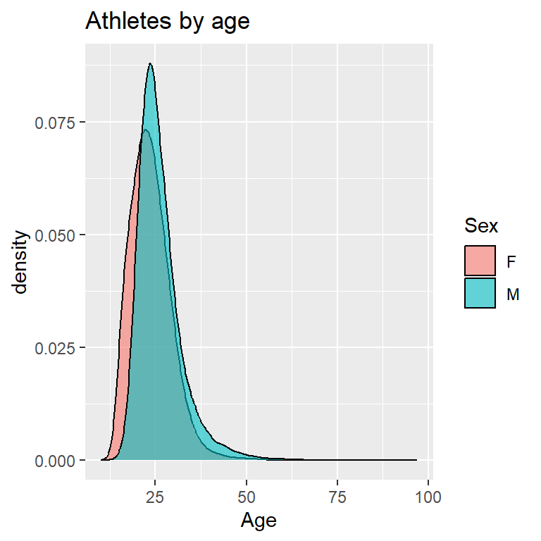

Code

# Plotting a kernel density graph for 'Height' variable

ggplot(olympic_data, aes(x = Height, fill = Sex)) +
  geom_density(adjust = 2, alpha = 0.6) + 
  labs(title = "Athletes by height")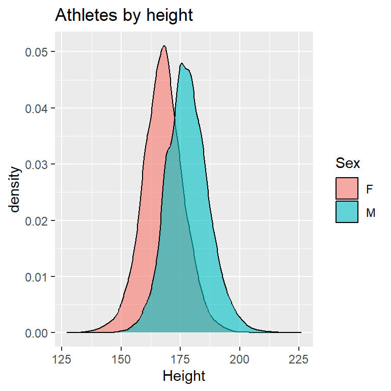

Code

# Plotting a kernel density graph for 'Weight' variable

ggplot(olympic_data, aes(x = Weight, fill = Sex)) +
  geom_density(adjust = 2, alpha = 0.6) + 
  labs(title = "Athletes by weight")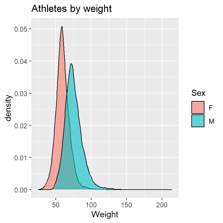

From the above plots, we can infer that the distribution of Height for both male and female athletes is symmetric which is little surprising. The distribution of Weight and Age for both male and female athletes are right-skewed indicating the mean>median.

The quantile statistics we get from the summary() for the variables ‘Age’, ‘Height’, and ‘Weight’ is not intuitive as the statistics are based on Male and Female athletes, and Summer and Winter games combined. I grouped the data based on ‘Season’ and ‘Sex’ and summarized the mean and median for the variables ‘Age’, ‘Height’, and ‘Weight’. The mean height and weight (175cm and 70kg respectively) obtained from the summary() on entire olympic_data is quite different from the mean height and weight (178cm and 75.4kg for male and 167cm and 59kg for female athletes) obtained from grouping the data based on season and sex. Hence, it is better to summarize the statistics for numerical variables after grouping the data as male and female quantile statistics will definitely be different.

Code

# Grouping the data based on 'Season' and 'Sex' and summarizing the mean and median for the variables 'Age', 'Height', and 'Weight'

olympic_data%>%
  group_by(Season, Sex)%>%
  summarise(mean_Age = round(mean(Age, na.rm = TRUE),digits =1),
            median_Age = median(Age, na.rm = TRUE),
            mean_Height = round(mean(Height, na.rm = TRUE),digits =1),
            median_Height = median(Height, na.rm = TRUE),
            mean_Weight = round(mean(Weight, na.rm = TRUE),digits =1),
            median_Weight = median(Weight, na.rm = TRUE))

I also grouped the data based on ‘Sex’ and summarized the mean and median for the variables ‘Age’, ‘Height’, and ‘Weight’. I did this to see how the mean and median of ‘Age’, ‘Height’, and ‘Weight’ variables changes with respect to grouping the data based on ‘Season’ and ‘Sex’. From the mean and median values below we can say that grouping the data based on season and sex or just by sex of the athletes does not change the statistics significantly. Therefore, for the remaining homework I will be focusing on the data grouped by ‘Sex’ variable.

Code

# Grouping the data based on 'Sex' and summarizing the mean and median for the variables 'Age', 'Height', and 'Weight'

olympic_data%>%
  group_by(Sex)%>%
  summarise(mean_Age = round(mean(Age, na.rm = TRUE),digits =1),
            median_Age = median(Age, na.rm = TRUE),
            mean_Height = round(mean(Height, na.rm = TRUE),digits =1),
            median_Height = median(Height, na.rm = TRUE),
            mean_Weight = round(mean(Weight, na.rm = TRUE),digits =1),
            median_Weight = median(Weight, na.rm = TRUE))

I have found the descriptive statistics for the numerical variables. Next, I will find the mode/frequency/distribution for the categorical variables like ‘Season’, ‘Sex’, ‘region’, ‘City’, ‘Sport’, ‘Event’, and ‘Medal’.

I found the frequency of values for variable ‘Season’ using the table(), the proportion of values using prop.table() and plotted a bar plot to represent the distribution of data observations for Season. I am using bar plots as I want to visualize the distribution of categorical variables. From the output of table(), prop.table() and the bar plot we know that we have 4 times more data observations for the Olympics Summer games compared to the Olympics Winter games. 82% of the data observations are for the Summer games and the remaining 18% is for the Winter games. One reason for this is that Winter Olympics has lesser teams/athletes and events (119 distinct events) compared to the Summer Olympics (651 distinct events).

Code

# Frequency/Proportion for variable 'Season'

table(olympic_data$Season)

Summer Winter 
221167  48564 

Code

prop.table(table(olympic_data$Season))

  Summer   Winter 
0.819954 0.180046 

Code

# Bar graph representing the distribution of data observations for Season.

library(ggplot2)

ggplot(olympic_data, aes(y = Season)) + 
  geom_bar(fill="#F8766D", width = 0.5) +
  labs(title = "Distribution of data observations for Season", 
       x = "Count", y = "Season")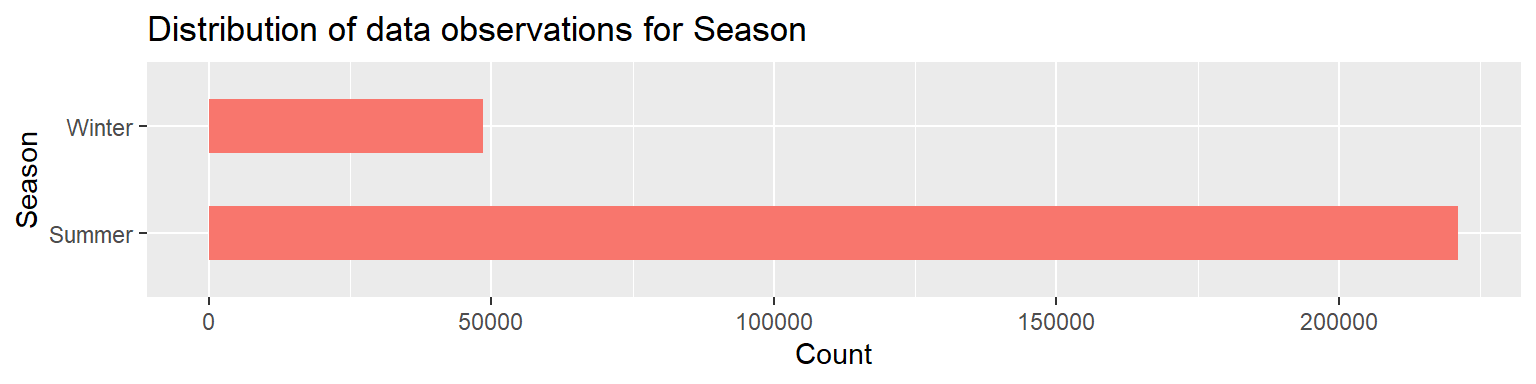

Code

# Displaying the count of distinct events in Winter Olympics

olympic_data%>%
  filter(Season=="Winter")%>%
  summarise(Distinct_Event = n_distinct(Event))

Code

# Displaying the count of distinct events in Summer Olympics

olympic_data%>%
  filter(Season=="Summer")%>%
  summarise(Distinct_Event = n_distinct(Event))

In order to further understand the reason behind lesser number of data observations for “Winter”, I decided to analyze the distribution of years and the distribution of Season over the years. I found the frequency of values for variable ‘Year’ using the table() and plotted a bar plot to represent the distribution of data observations for years 1896 - 2016.

Code

# Frequency for variable 'Year'

table(olympic_data$Year)

 1896  1900  1904  1906  1908  1912  1920  1924  1928  1932  1936  1948  1952 
  380  1898  1301  1733  3069  4040  4292  5570  5238  2817  7146  7383  9358 
 1956  1960  1964  1968  1972  1976  1980  1984  1988  1992  1994  1996  1998 
 6434  9235  9480 10479 11959 10502  8937 11588 14676 16413  3160 13780  3605 
 2000  2002  2004  2006  2008  2010  2012  2014  2016 
13821  4109 13443  4382 13602  4402 12920  4891 13688 

Code

# Bar graph representing the distribution of data observations over Year

library(ggplot2)

ggplot(olympic_data, aes(x = Year)) + 
  geom_bar(fill="#00BFC4") +
  ylim(0,20000) +
  labs(title = "Distribution of data observations over Year", 
       x = "Year", y = "Count") +
  geom_text(stat='count', aes(label=..count..), hjust = -0.3, size = 3, angle = 90)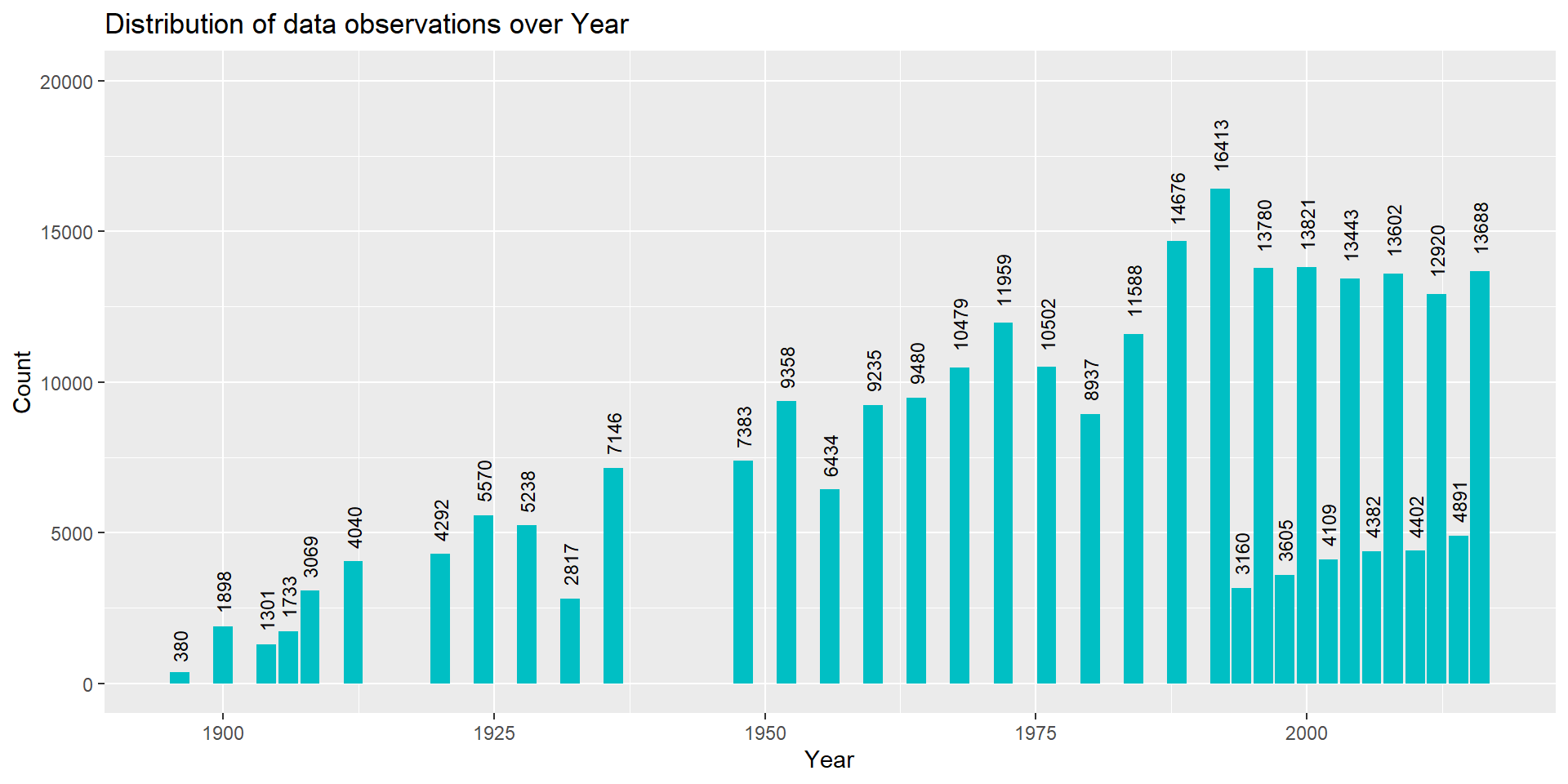

From the output of table() function and the bar plot we can observe that the year 1896 has the least number of data observations and the year 1992 has the most number of data observations. This is because the year 1896 had the least number of events (43) and the year 1992 had the most number of events (314) in the Olympic games which can be observed from the bar plot below. The Olympic games were held once every 4 years from 1896 - 1992 before staggering into Winter Olympics from 1994 and Summer Olympics from 1996. However, we can notice that there are few gaps in the bar plot for years 1916, 1940, and 1944. All three Olympic games were cancelled due to the World War. There was a Summer Olympics known as the Intercalated Olympic Games held between 1904 and 1908 in the year 1906. The Intercalated Olympic Games were conceived as a series of international athletics competitions that would take place every four years, halfway between the actual Olympics, and would always be hosted in Athens. However, they were only held once, in 1906 and discontinued after that as the athletes did not have enough time to prepare for the Games.

Code

# Grouping the data by 'Year' and summarizing for the count of distinct values for 'Event' in each group

event_over_year <- olympic_data%>%
  group_by(Year)%>%
  summarise(Distinct_Event = n_distinct(Event))

# Bar plot representing the number of distinct events over the years

ggplot(event_over_year, aes(x = Year, y = Distinct_Event)) + 
  geom_bar(fill="#CD9600", stat = "identity") +
  ylim(0,350) +
  labs(title = "Distribution of Distinct Events over Years", 
       x = "Year", y = "Count of Distinct Events") +
  geom_text(aes(label=Distinct_Event), hjust = -0.3, size = 3, angle = 90)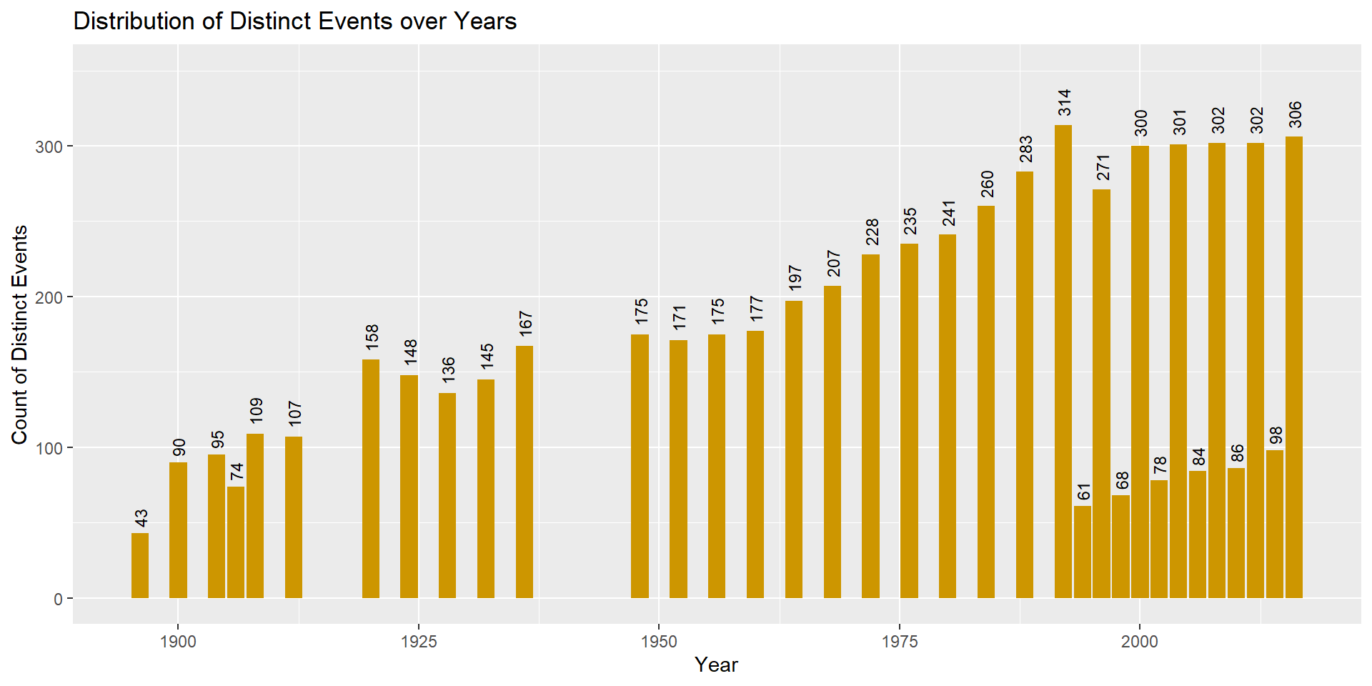

The distribution of Season over the Year plot below conveys that the ‘Winter’ games originated in 1924. Since the ‘Summer’ games originated way before in 1896 we have more observations for ‘Summer’ games in addition to the reason of more number of events. From 1924 - 1992, both ‘Summer’ and ‘Winter’ Games were held on the same year. The Winter olympics has taken place in 22 distinct years and the Summer Olympics in 29 distinct years.

Code

# Stacked bar graph representing the distribution of Season over the years 

ggplot(olympic_data, aes(x = Year, fill = Season)) + 
  geom_bar() +
  labs(title = "Distribution of Season over Year", 
       x = "Year", y = "Count")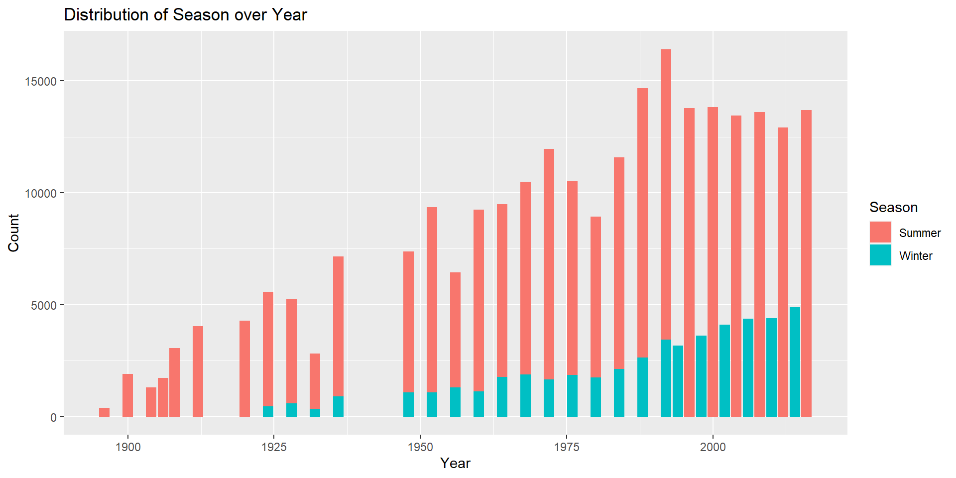 

Code

# Displaying the count of distinct years in Winter Olympics

olympic_data%>%
  filter(Season=="Winter")%>%
  distinct(Year)

Code

# Displaying the count of distinct years in Summer Olympics

olympic_data%>%
  filter(Season=="Summer")%>%
  distinct(Year)

I grouped the data by ‘Year’ and ‘Sex’ variables and summarized the count of unique athletes in order to find the distribution of ‘Sex’ over the years in the Olympic games. I plotted a line plot to represent the distribution of data observations for Sex.

Code

# Grouping by 'Year' and 'Sex' and summarizing the count of unique Athletes

year_sex <- olympic_data %>% 
  group_by(Year, Sex) %>%
  summarize(athlete_count = length(unique(ID)))%>%
  mutate(Year = as.integer(Year))
year_sex

Code

# Line plot representing the count of athletes over the years grouped by Sex

ggplot(year_sex, aes(x = Year, y = athlete_count, group = Sex, color = Sex)) + 
  geom_line() +
  geom_point() +
  geom_smooth() +
  labs(title = "Distribution of Athletes over the years grouped by Sex", 
       x = "Year", y = "Count of Athletes")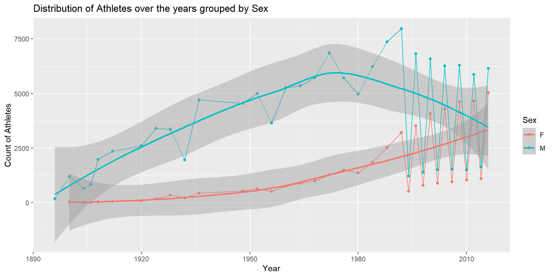

The above line plot can be used to answer the research question: What is the ratio of male to female athletes participating in the Olympic games and has gender equality of athletes participating increased over the past 120 years? The participation of female athletes in Olympics has gradually increased over the past 120 years (which is clear from the trend line). The line plot above indicates that the 1896 Olympics did not have any Female athletes. From 1900 - 1960, the growth of female athletes in the Olympics was slow. After 1960, the Olympics had increased participation of female athletes which is a good sign that more countries are supporting female athletes (may also be a tactic to win more medals in women’s events and increase the medal tally). In the 2016 Rio Olympics, about 40% of the athletes were Female. After 1992, the ratio of male to female athletes has decreased. This can be seen from the gap between the trend lines decreasing after 1992. In future, we can expect the ratio of male to female athletes to be 1:1.

Next, I grouped the data by ‘region’ variable and summarized the count of distinct ‘Year’ to find the number of times a region/country has participated in the Olympics. For the past 120 years (1896 - 2016), there have been 35 Olympic Games including both Summer and Winter.

Code

# Grouping by 'region' and summarizing the count of distinct 'Year'

region_participation <- olympic_data %>% 
  group_by(region) %>%
  summarize(participation_count = length(unique(Year)))
region_participation

I plotted a bar plot to represent the participation of region in the Olympics. Since, there are 209 regions, I sorted the region_participation in increasing order of participation_count and took a subset of the data which had participation_count >= 30. This accounted to 21 observations with 7 regions having participated in all the Olympic Games from the beginning. The 7 regions are USA, UK, Switzerland, Italy, Greece, France, and Australia.

Code

# Bar graph representing the participation of region

region_participation <- region_participation%>%
  arrange(participation_count)%>%
  filter(participation_count>=30)

ggplot(region_participation, aes(x = reorder(region, participation_count), y = participation_count)) + 
  geom_bar(fill="#00BE67", stat = "identity", width = 0.8) +
  scale_y_continuous(limits = c(0, 35), breaks = seq(0, 35, by = 2)) +
  labs(title = "Participation of region in the Olympics", 
       x = "Region", y = "Number of times participated") +
  theme(axis.text.x=element_text(angle=90, hjust=1))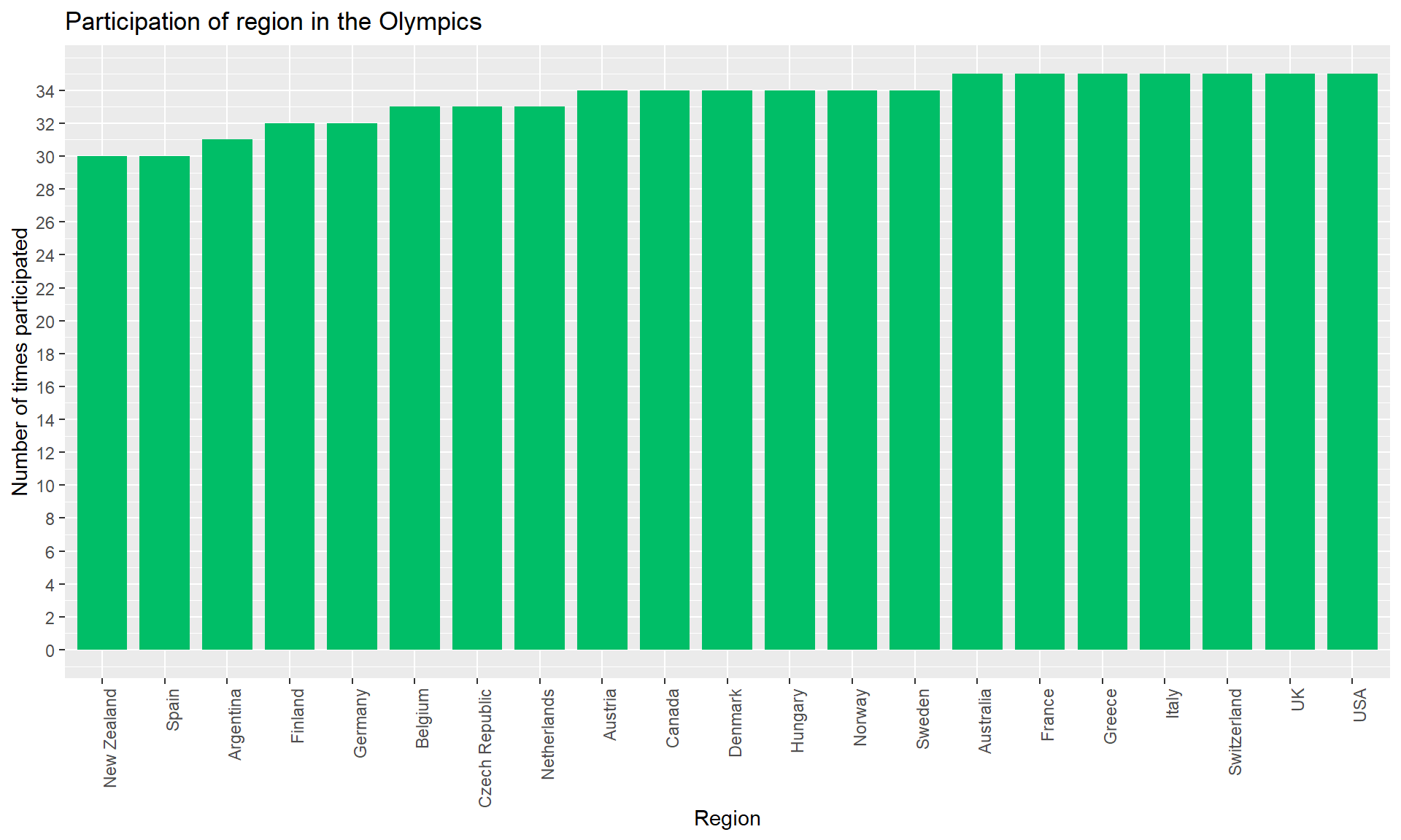

Next, I grouped the data by ‘City’ variable and summarized the count of distinct ‘Year’ to find the number of times a city has hosted the Olympic Games. The host city is elected by a majority of the votes cast by secret ballot by the members of the IOC. Each active member has one vote.

Code

# Grouping by 'City' and summarizing the count of distinct 'Year'

host_city <- olympic_data %>% 
  group_by(City) %>%
  summarize(host_city_count = length(unique(Year)))
host_city

I plotted a bar plot to represent the distribution of host city in the Olympics. There are 42 host cities and I sorted the host_city in increasing order of host_city. The cities Athina (alternate name for Athens) and London have hosted the Olympic games thrice and the cities Innsbruck, Paris, Lake Placid, Los Angeles, Sankt Moritz, and Stockholm have hosted the Olympics twice each. The remaining cities have hosted the Olympics only once from 1896 - 2016.

Code

# Bar graph representing the distribution of Host City

host_city <- host_city%>%
  arrange(host_city_count)

ggplot(host_city, aes(x = City, y = host_city_count)) + 
  geom_bar(fill="#8494FF", stat = "identity", width = 0.5) +
  labs(title = "Distribution of Host City in the Olympics", 
       x = "City", y = "Number of times hosted") +
  theme(axis.text.x=element_text(angle=90, hjust=1)) +
  geom_text(aes(label=host_city_count), vjust = -0.5, size = 3)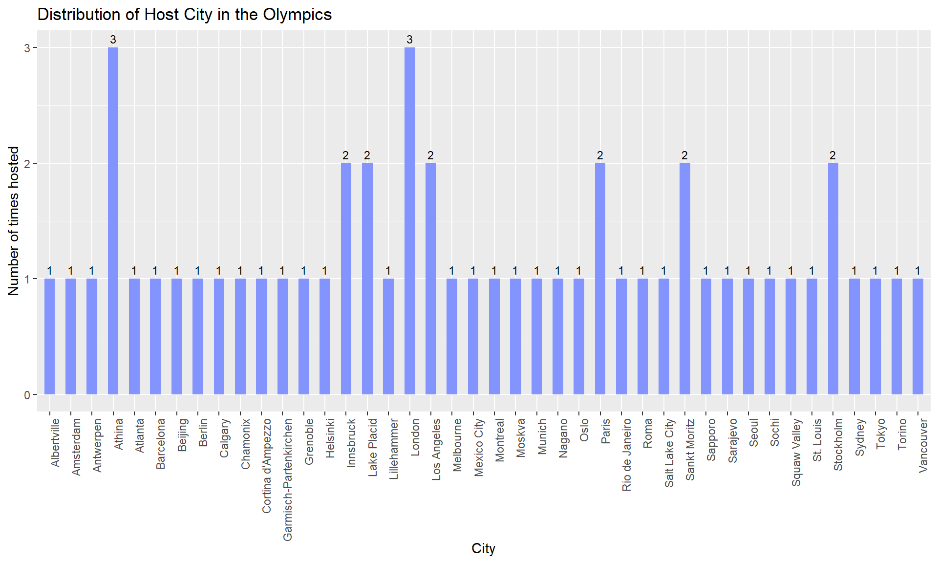

Next, I grouped the data by ‘Sport’ variable and summarized the count of distinct ‘Year’ to find the number of times a Sport has been played in the Olympic Games.

Code

# Grouping by 'Sport' and summarizing the count of distinct 'Year'

sport_year <- olympic_data %>% 
  group_by(Sport) %>%
  summarize(sport_count = length(unique(Year)))
sport_year

I plotted a bar plot to represent the distribution of Sport in the Olympics. There are 66 distinct sports and I sorted the sport_year in increasing order of ‘sport_count’. The sports Athletics, Cycling, Fencing, Gymnastics, and Swimming has had events in 29 Olympic Games followed by Rowing and Wrestling in 28 Olympic Games. One reason, for the Sports to have more occurrences in the Olympic Games is that they may have been introduced in the initial Olympic Games. There are few Sports which were introduced as an Olympic sport at a later stage. For example, Taekwondo was introduced as an Olympic Sport in the 2000s.

Code

# Bar graph representing the distribution of Sport

sport_year <- sport_year%>%
  arrange(sport_count)

ggplot(sport_year, aes(x = Sport, y = sport_count)) + 
  geom_bar(fill="#E68613", stat = "identity", width = 0.5) +
  labs(title = "Distribution of Sport in the Olympics", 
       x = "Sport", y = "Frequency") +
  theme(axis.text.x=element_text(angle=90, hjust=1)) +
  geom_text(aes(label=sport_count), vjust = -0.5, size = 3)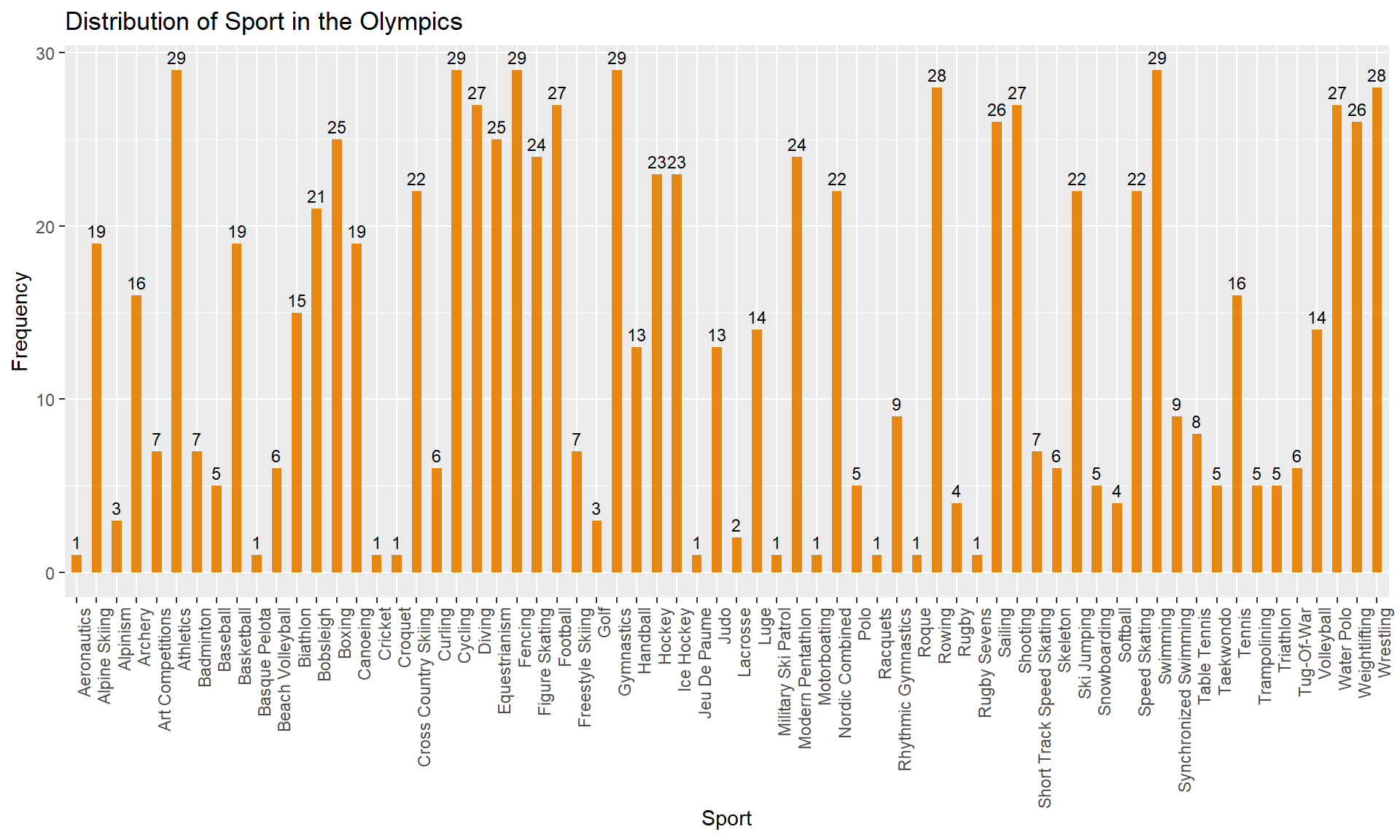

Finally, I found the frequency of values for variable ‘Medal’ using the table() and plotted a bar plot to represent the distribution of data observations for Medal grouped by Sex. From the output of table() and the bar plot we know that the number of bronze, silver and gold medals are approximately 13,000 each and male athletes have won more mdeals compared to female athletes. Out of the 269,731 observations in olympic_data, about 39,772 observations are for medal winning athletes.

Code

# Frequency for variable 'Medal'

table(olympic_data$Medal)

  Bronze     Gold No Medal   Silver 
   13295    13369   229959    13108 

Code

prop.table(table(olympic_data$Medal))

    Bronze       Gold   No Medal     Silver 
0.04928985 0.04956420 0.85254939 0.04859656 

Code

# Bar graph representing the distribution of data observations for Medal grouped by Sex

ggplot(olympic_data, aes(y = Medal)) + 
  geom_bar(fill="#7CAE00", width = 0.5) +
  facet_grid(~Sex) +
  labs(title = "Distribution of data observations for Medal grouped by Sex", 
       x = "Count", y = "Medal")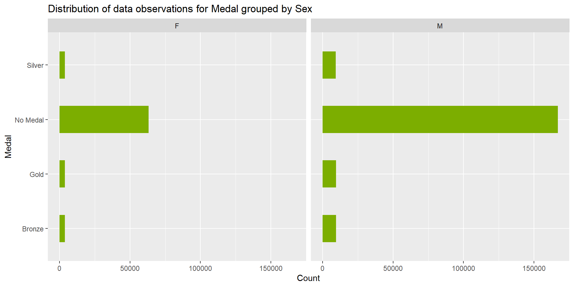

I also filtered the olympic_data to remove the observations which had the value ‘No Medal’ and plotted a stacked bar graph to represent the distribution of Medal over Year. This helps us to verify that the ratio of bronze:silver:gold medals over the years is almost 1:1:1. This makes sense as each event will have bronze, silver and gold medals awarded.

Code

# Stacked bar graph representing the distribution of Medal over Year

medal_year <- olympic_data%>%
  filter(Medal!="No Medal")

ggplot(medal_year, aes(x = Year, fill = Medal)) + 
  geom_bar() +
  labs(title = "Distribution of Medal over Year", 
       x = "Count", y = "Year")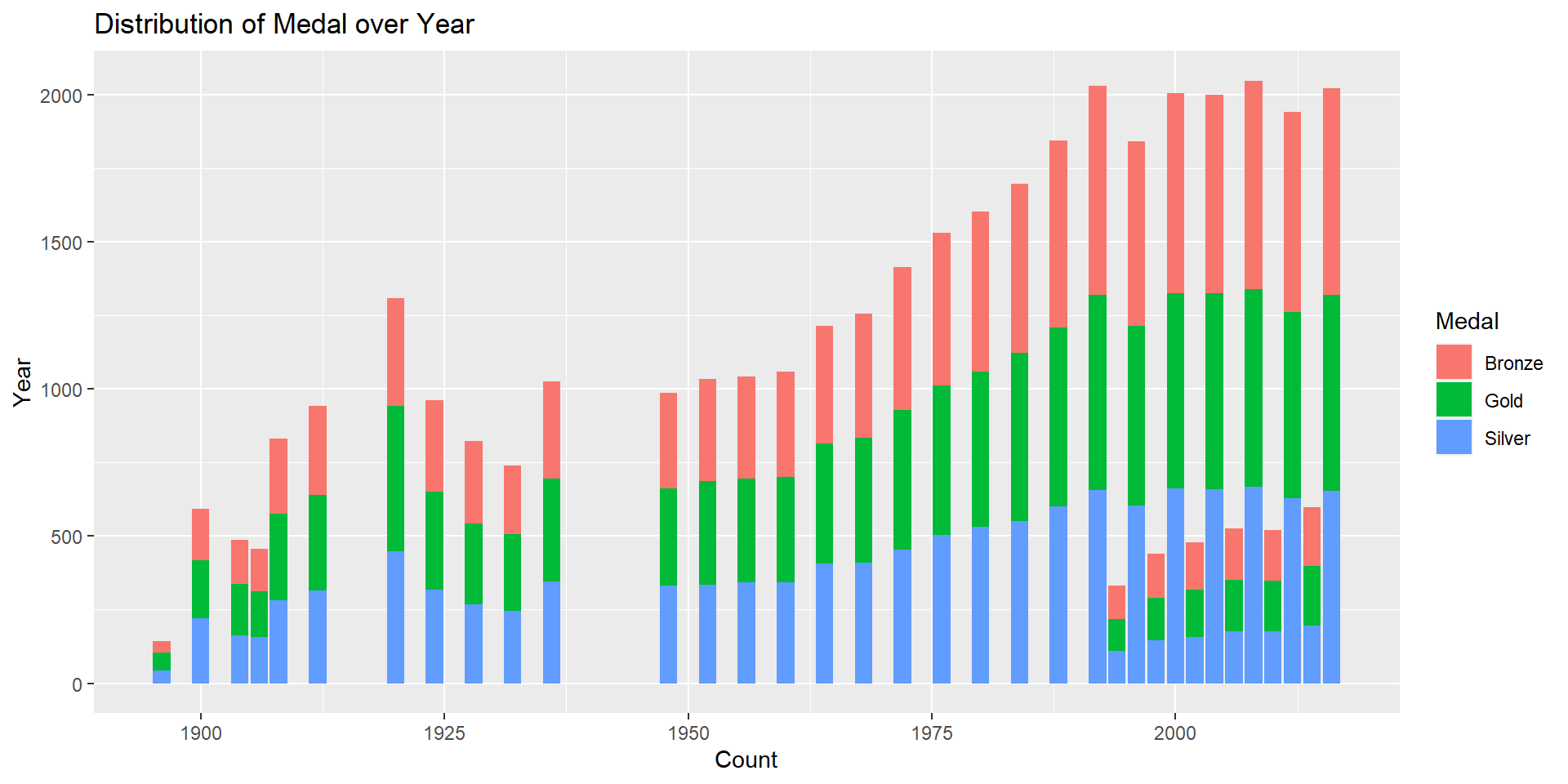

Visualizations

There are few research questions which can be answered using the cleaned ‘olympic_data’ dataset and visualizations.

Top Medal Winning Athletes

Research question: Which female athlete and male athlete have won the most number of medals in the Olympic Games held from 1896 - 2016 and analyze their distribution of winning medals? Which female and male athlete have won the most number of medals in a single year of the Olympic Games? What is the distribution of medals won by the top 5 medal winning athletes over the years?

As the first step to answer this question, I split the olympic_data into 2 separate tibbles - one containing information about female athletes and another one about male athletes.

Code

# Splitting into female_olympic_data and male_olympic_data

female_olympic_data <- olympic_data%>%
  filter(Sex=="F")
male_olympic_data <- olympic_data%>%
  filter(Sex=="M")

# Filtering the 'No Medal' observations, grouping by 'Name', performing pivot_wider, summarizing the count of medals won, sorting based on total medals and finding the top 5 medal winning female athletes

max_medal_female <- female_olympic_data %>%
  filter(Medal!="No Medal")%>%
  group_by(Name) %>%
  count(Medal)%>%
  pivot_wider(names_from = Medal, values_from = n)%>%
  mutate(Total_Medal = sum(Gold, Silver, Bronze, na.rm=TRUE))%>%
  arrange(desc(Total_Medal))%>%
  head(5)
max_medal_female

Code

# Filtering the 'No Medal' observations, grouping by 'Name', performing pivot_wider, summarizing the count of medals won, sorting based on total medals and finding the top 5 medal winning male athletes

max_medal_male <- male_olympic_data %>%
  filter(Medal!="No Medal")%>%
  group_by(Name) %>%
  count(Medal)%>%
  pivot_wider(names_from = Medal, values_from = n)%>%
  mutate(Total_Medal = sum(Gold, Silver, Bronze, na.rm=TRUE))%>%
  arrange(desc(Total_Medal))%>%
  head(5)
max_medal_male

In order to find the top 5 medal winning female athletes, I filtered the ‘No Medal’ observations from female_olympic_data, grouped by ‘Name’, found count of medals for Gold, Silver,and Bronze, performed pivot_wider to get one observation for each athlete, mutated ‘Total_Medal’ variable by adding Gold+Silver+Bronze medals, sorted based on ‘Total_Medal’ in descending order and extracted the top 5 observations. The same steps were repeated for finding the top 5 medal winning male athletes. Larysa Semenivna Latynina (Diriy-) is the female athlete that has won the most number of medals (18) in Olympics in the past 120 years. She represented the Soviet Union team for the Gymnastic Sport and won 9 Gold, 5 Silver and 4 Bronze medals. Michael Fred Phelps, II is the male athlete that has won the most number of medals (28) in Olympics in the past 120 years. He represented team USA for the Swimming Sport and won 23 Gold, 3 Silver and 2 Bronze medals.

Code

# Distribution of Medals won by top 5 medal winning female athletes over the years

top_medal_female <- female_olympic_data%>%
  filter(Name %in% max_medal_female$Name)%>%
  filter(Medal!="No Medal")%>%
  group_by(Name, Year)%>%
  count(Medal)%>%
  pivot_wider(names_from = Medal, values_from = n)%>%
  mutate(Total_Medal = sum(Gold, Silver, Bronze, na.rm=TRUE))%>%
  arrange(desc(Total_Medal))

# Line plot representing the distribution of Medals over the years grouped by Athlete Name

ggplot(top_medal_female, aes(x = Year, y = Total_Medal, group = Name, color = Name)) + 
  geom_line() +
  geom_point() +
  labs(title = "Distribution of Medals over the years grouped by Athlete Name (Female)", 
       x = "Year", y = "Total Medals won")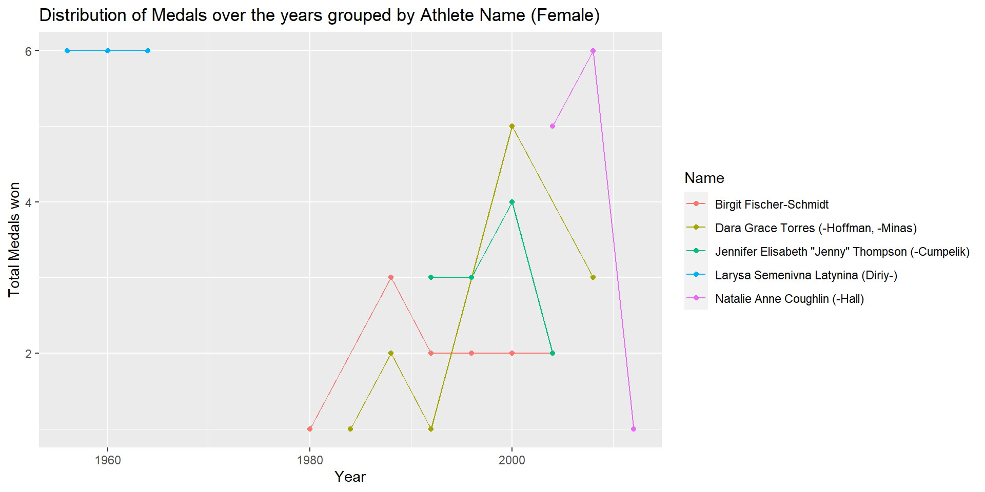

Code

# Distribution of Medals won by top 5 medal winning male athletes over the years

top_medal_male <- male_olympic_data%>%
  filter(Name %in% max_medal_male$Name)%>%
  filter(Medal!="No Medal")%>%
  group_by(Name, Year)%>%
  count(Medal)%>%
  pivot_wider(names_from = Medal, values_from = n)%>%
  mutate(Total_Medal = sum(Gold, Silver, Bronze, na.rm=TRUE))%>%
  arrange(desc(Total_Medal))

# Line plot representing the distribution of Medals over the years grouped by Athlete Name

ggplot(top_medal_male, aes(x = Year, y = Total_Medal, group = Name, color = Name)) + 
  geom_line() +
  geom_point() +
  labs(title = "Distribution of Medals over the years grouped by Athlete Name (Male)", 
       x = "Year", y = "Total Medals won")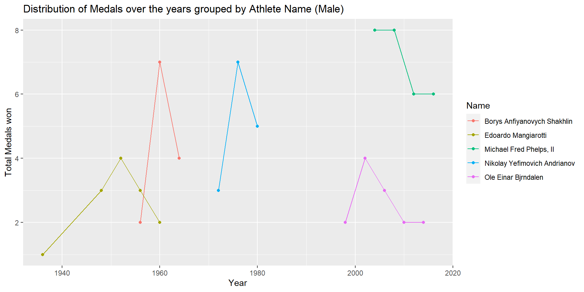

From the above line plots, we can analyze the distribution of medals won by the top 5 medal winning athletes. Semenivna Latynina (Diriy-) won 6 medals each in years 1956, 1960, and 1964. Michael Fred Phelps, II won 8,8,6, and 6 medals in years 2004, 2008, 2012 and 2016 respectively.

Next, I have to find the female and male athlete who won the most number of medals in a single year of the Olympic Games.

Code

# Filtering the 'No Medal' observations, grouping by 'Year' and 'Name', performing pivot_wider, summarizing the count of medals won, sorting based on total medals and finding the top 6 medal winning female athletes

max_medal_female_year <- female_olympic_data %>%
  filter(Medal!="No Medal")%>%
  group_by(Year,Name) %>%
  count(Medal)%>%
  pivot_wider(names_from = Medal, values_from = n)%>%
  mutate(Total_Medal = sum(Gold, Silver, Bronze, na.rm=TRUE))%>%
  arrange(desc(Total_Medal), desc(Gold))%>%
  head(6)
max_medal_female_year

Code

# Filtering the 'No Medal' observations, grouping by 'Year' and 'Name', performing pivot_wider, summarizing the count of medals won, sorting based on total medals and finding the top 6 medal winning male athletes

max_medal_male_year <- male_olympic_data %>%
  filter(Medal!="No Medal")%>%
  group_by(Year, Name) %>%
  count(Medal)%>%
  pivot_wider(names_from = Medal, values_from = n)%>%
  mutate(Total_Medal = sum(Gold, Silver, Bronze, na.rm=TRUE))%>%
  arrange(desc(Total_Medal), desc(Gold))%>%
  head(5)
max_medal_male_year

Mariya Kindrativna Horokhovska is the female athlete that won the highest number of medals (7) in a single year 1952 of the Olympic Games. She won 2 Gold and 5 Silver medals. Michael Fred Phelps, II is the male athlete that won the highest number of medals (8) in 2 consecutive Olympics held in years 2008 and 2004. He won 8 Gold medals in 2008 and 6 Gold and 2 Bronze medals in 2004. Aleksandr Nikolayevich Dityatin is another male athlete who won 8 medals in the year 1980. He won 3 Gold, 4 Silver and 1 Bronze medals representing team Soviet Union for Sport Gymnastics.

Top Medal Winning Region

Research Question: **Which region has won the highest number of medals in the Olympic history? What is the distribution of the top 10 medal winning regions?

For answering this question, I will be working with the olympic_data.

Code

# Find total number of medals won in Olympics history

total_medal <- olympic_data%>%
  filter(Medal!="No Medal")%>%
  count(Medal)%>%
  pivot_wider(names_from = Medal, values_from = n)%>%
  mutate(Total_Medal = sum(Gold, Silver, Bronze, na.rm=TRUE))

# Filtering the 'No Medal' observations, grouping by 'region', performing pivot_wider, summarizing the count of medals won, sorting based on total medals and finding the top 10 medal winning regions

max_medal_region <- olympic_data %>%
  filter(Medal!="No Medal")%>%
  group_by(region) %>%
  count(Medal)%>%
  pivot_wider(names_from = Medal, values_from = n)%>%
  mutate(Total_Medal = sum(Gold, Silver, Bronze, na.rm=TRUE))%>%
  arrange(desc(Total_Medal))%>%
  head(10)%>%
  mutate(Medal_Won_Percentage = round(Total_Medal/total_medal$Total_Medal,digits = 2)*100)
max_medal_region

In order to find the top 10 medal winning regions, I filtered the ‘No Medal’ observations from olympic_data, grouped by ‘region’, found count of medals for Gold, Silver,and Bronze, performed pivot_wider to get one observation for each region, mutated ‘Total_Medal’ variable by adding Gold+Silver+Bronze medals, sorted based on ‘Total_Medal’ in descending order and extracted the top 10 observations. USA has won the highest number of medals in the Olympics history followed by Russia and Germany. USA has won a total of 5637 medals including 2638 Gold, 1641 Silver, and 1358 Bronze medals. A total of 39,772 medals have been awarded in the Olympics history. I also computed the percentage of medals won out of the total medals by the top 10 medal winning regions. USA has won 14% of the total medals in Olympics.

Next, I plotted a grouped bar graph to visualize the distribution of medals for the top 10 medal winning regions. Grouped bar chart enables us to compare the different medals (Gold, Silver and Bronze) won by a region within itself and among other regions also. For this purpose, I used the medal_year which I had created earlier while doing descriptive statistics for ‘Medal’ variable.

Code

# Distribution of Medals won by top 10 medal winning regions

top_medal_region <- medal_year%>%
  filter(region %in% max_medal_region$region)%>%
  filter(Medal!="No Medal")

# Grouped bar graph representing the distribution of Medals for the top 10 medal winning regions

ggplot(top_medal_region, aes(x = region, fill = Medal)) + 
  geom_bar(position = "dodge",width = 0.8) +
  labs(title = "Distribution of Medals for top 10 medal winning regions", 
      x = "Region", y = "Total Medals won")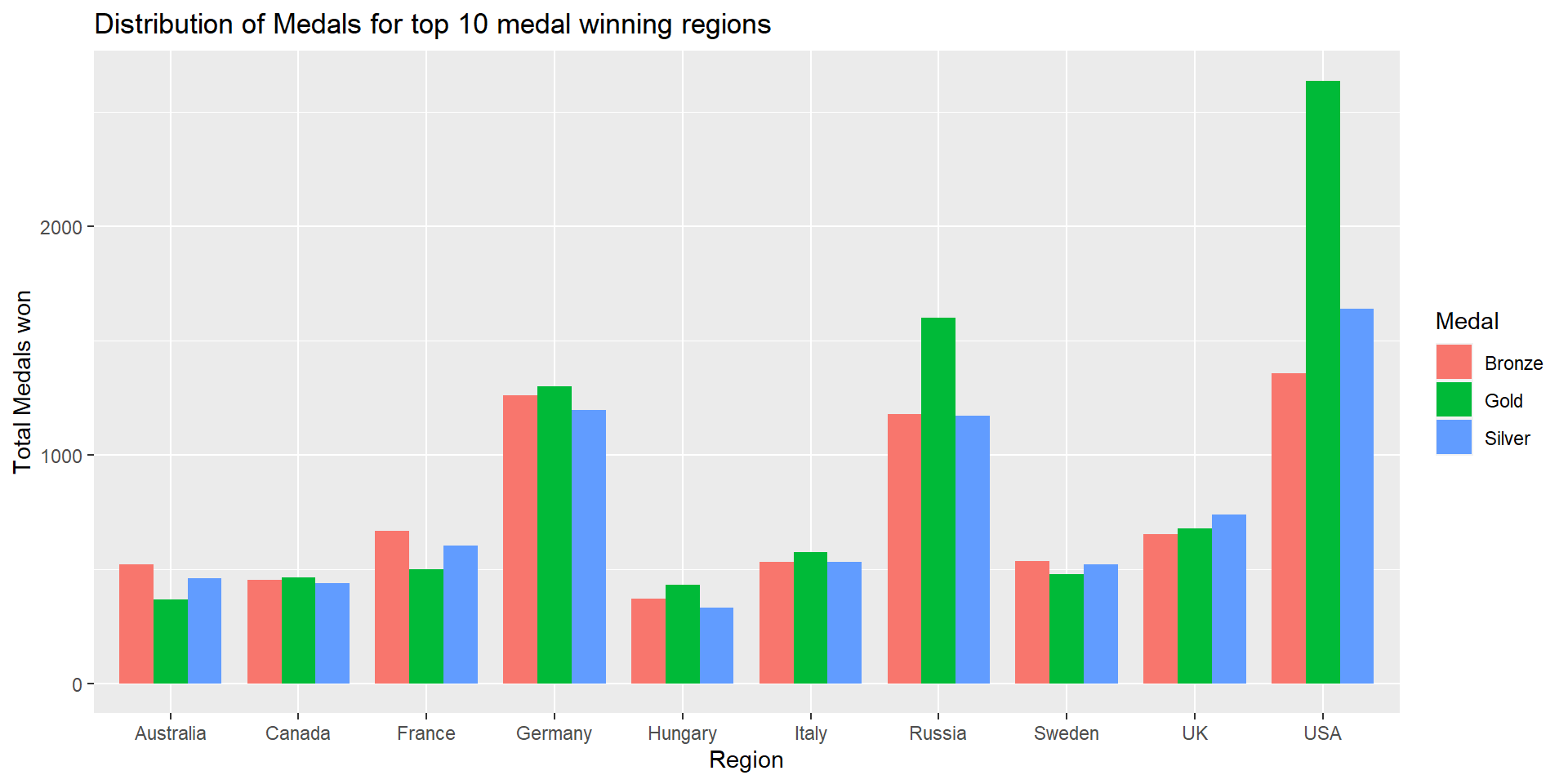

From the grouped bar chart, we can infer that the top 3 medal winning regions have more Gold medals compared to Silver and Bronze.

Analyzing Age/Height/Weight of Athletes over the years

Research question: Has there been a significant change in the age/height/weight of athletes participating in the various events over the years?

I plotted a box plot to represent the Height of Athletes over the years grouped by ‘Sex’ after dropping all the observations with missing values for ‘Height’ and ‘Weight’. After plotting, I noticed that most of the observations for Female athletes has missing ‘Height’ or ‘Weight’ values before the year 1920. Hence, I plotted the box plot starting after 1920. For the purpose of plotting the box plots, I converted the ‘Year’ variable to factor.

Code

# Box plot representing the Height of Athletes over the years grouped by Sex

olympic_data %>% 
  filter(!is.na(Height), !is.na(Weight))%>%
  filter(Year>1920)%>%
  ggplot(aes(x=as.factor(Year), y=Height, fill=Sex)) +
  geom_boxplot() +
  labs(title = "Height(cm) of Athletes over the years", 
       x = "Year", y = "Height(cm)") +
  theme(axis.text.x=element_text(angle=90, hjust=1))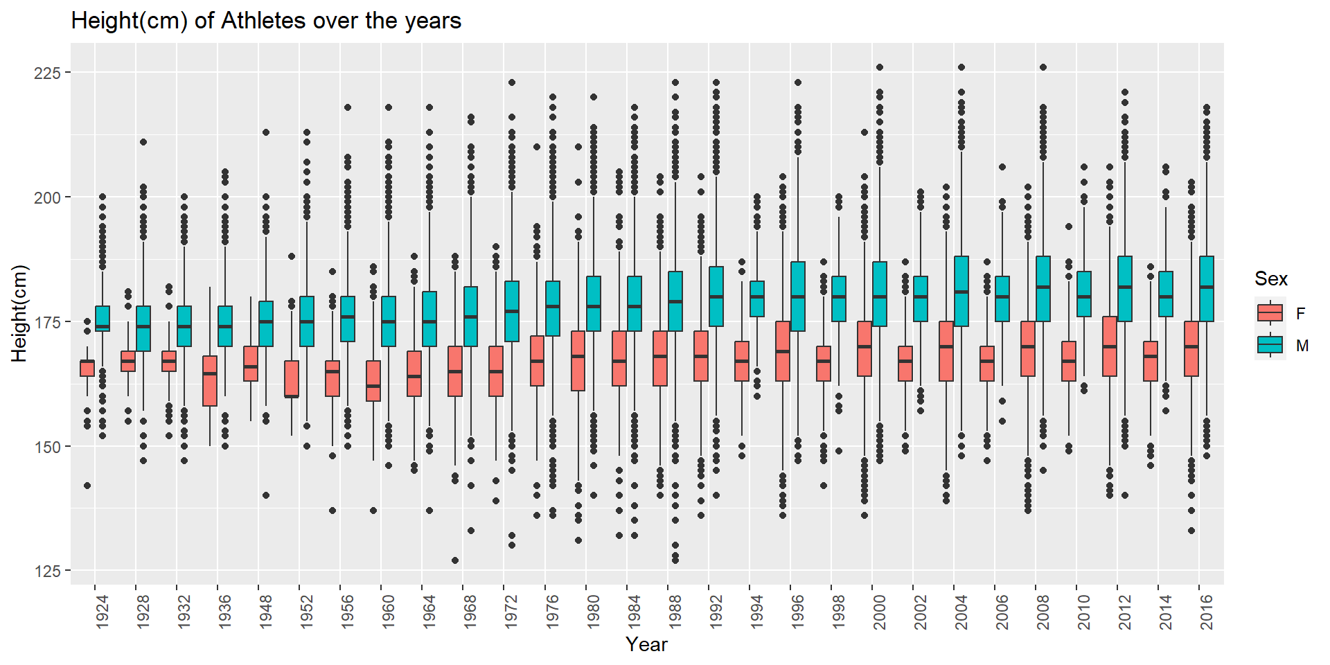

From the above box plot, we can observe that for both male and female athletes the height has gradually increased over the years. For each year, we can see few outliers. The Athletes with extremely short height usually participate in Gymnastics and Boxing Sports and the extremely tall athletes usually participate in Sports like Basketball and Volleyball.

Next, I plotted a box plot to represent the Height of Athletes over the years grouped by ‘Sex’ after dropping all the observations with missing values for ‘Height’ and ‘Weight’. After plotting, I noticed that most of the observations for Female athletes has missing ‘Height’ or ‘Weight’ values before the year 1920. Hence, I plotted the box plot starting after 1920.

Code

# Box plot representing the Weight of Athletes over the years grouped by Sex

olympic_data %>% 
  filter(!is.na(Height), !is.na(Weight))%>%
  filter(Year>1920)%>%
  ggplot(aes(x=as.factor(Year), y=Weight, fill=Sex)) +
  geom_boxplot() +
  labs(title = "Weight(kg) of Athletes over the years", 
       x = "Year", y = "Weight(kg)") +
  theme(axis.text.x=element_text(angle=90, hjust=1))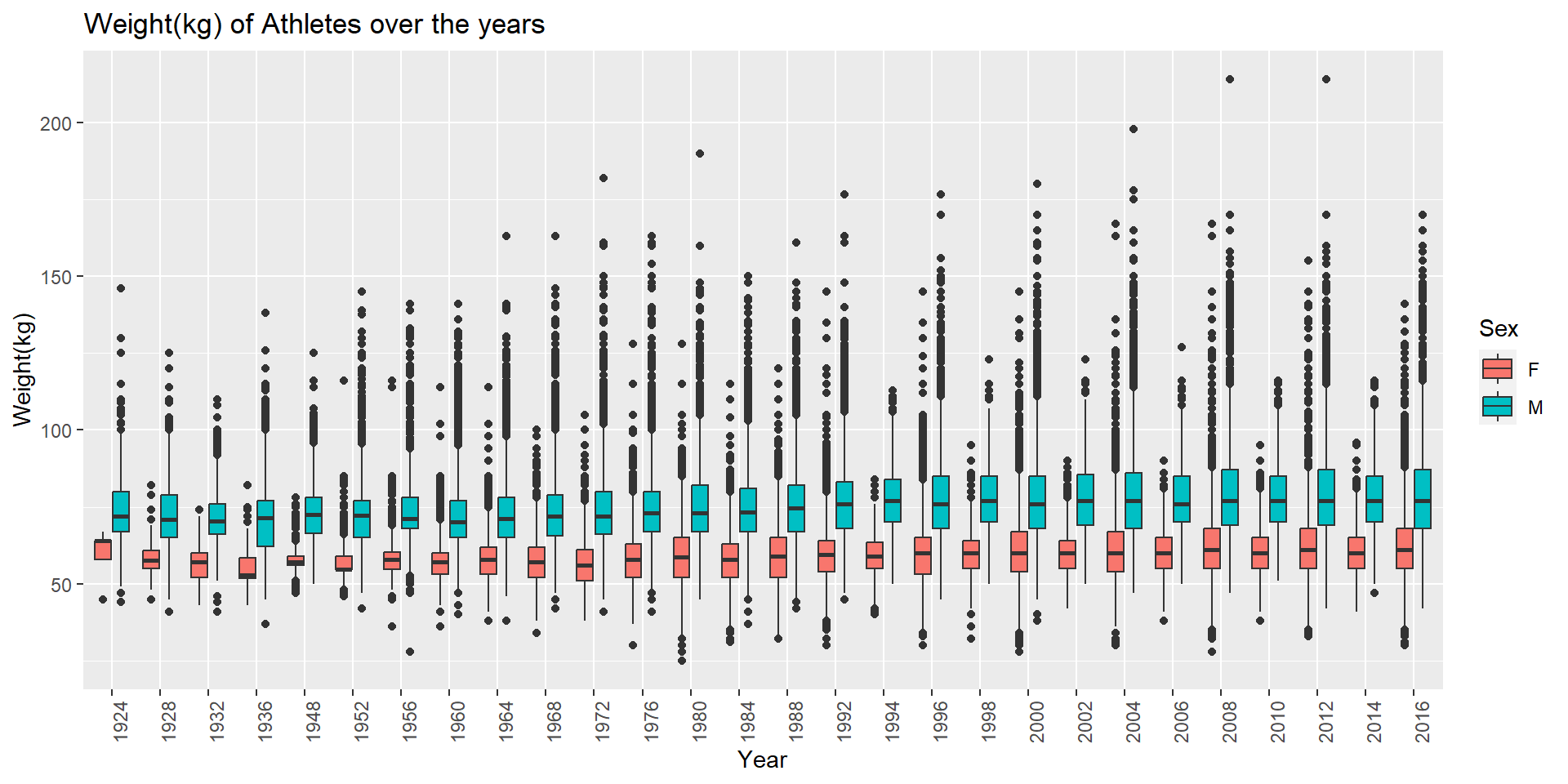

From the above box plot, we can observe that for both male and female athletes the Weight has gradually increased over the years. For each year, we can see few outliers. The Athletes with extremely low weight usually participate in Gymnastics Sport and the extremely heavy weight athletes usually participate in Sports like Judo, Wrestling, and Weightlifting.

Code

# Box plot representing the Age of Athletes over the years grouped by Sex

olympic_data %>% 
  ggplot(aes(x=as.factor(Year), y=Age, fill=Sex)) +
  geom_boxplot() +
  labs(title = "Age of Athletes over the years", 
       x = "Year", y = "Age") +
  theme(axis.text.x=element_text(angle=90, hjust=1))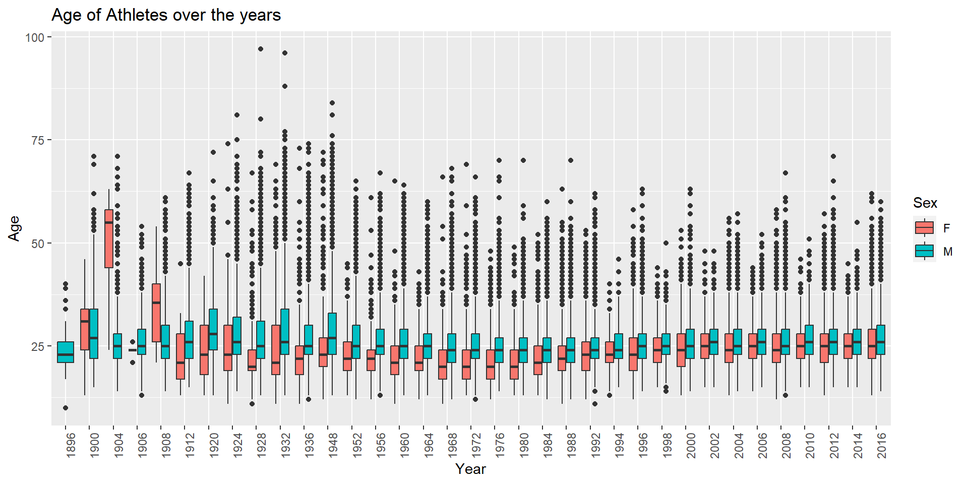

The age distribution fluctuates in the starting few years and gradually increases after the year 1964. The age distribution for female athletes in the year 1904 is very different from the remaining years. There are few instances where the Age of athletes is above 75 which is quite abnormal for participating in Sports. I looked into the data to analyze the reasons behind these.

Code

# Displaying the data observations of Female athletes for the year 1904

olympic_data%>%
  filter(Sex=="F")%>%
  filter(Year==1904)

All the 16 female athletes in the 1904 Olympics, participated in the Archery sport and represent the region USA.

Code

# Displaying the data observations of athletes >= 75 Age

olympic_data%>%
  filter(Age>=75)

The 14 athletes with Age >= 75 participated in the ‘Art Competitions’ Sport for Olympic Games which makes sense as Art Competitions does not require mcuh stamina and adrenaline like other sports. The Art Competitions were held at the Olympics from 1912 - 1948.

Reflection

Process

I started the project by briefly exploring the data and understanding the datatype of each variable. I performed data cleaning on both the datasets and handled missing values for Height, Weight and Age using the mean value grouped by Season, Sex, Year and Event (as it did not make sense to find the mean Age/Height/Weight over the entire data), and for the region using the notes. After cleaning both the datasets, I joined the datasets using NOC code as the key. I used this clean dataset for further analysis. The descriptive statistics gave me insights about the distribution of the variables for Male and Female athletes. Following this, I used visualizations to answer few research questions about the athletes who won the most medals and the distribution of the top 5 medal winning Male and Female athletes. I was also able to find the 3 regions which have won the most medals (accounting to around 35% of the total medals in the Olympic Games). I was able to analyze whether there has been a significant change in the age/height/weight of athletes participating in the various events over the years? The current dataset does not have any information about the coordinates of the regions which makes it impossible to visualize the representation of each region in the Olympic Games for a given year. It would require extra effort to map each region to their corresponding latitude and longitude form the world map.

Future Work

Analyzing Host City Advantage

Research question: Does the host city have any advantage in Olympic games in terms of winning more medals? (i.e does the Team/NOC/region win more medals when the City hosting the Olympic games is in that region)

As part of the next steps, I would like to find whether hosting the Olympics gives the region an added advantage in terms of winning more medals. One reason for this may be that, since the host city is constantly in the spotlight during the Olympics it would be bad publicity if the City does not perform well in the Olympics. There is a possibility that the region Government allocates more resources for training their athletes to perform well and win more medals. For finding this out, we would have to map the host city with the region and find the average medals won by the region in the years it did not host the Olympics and compare it with the medals won during the year it hosted the Olympics Games. There is also a possibility, that the hosting cities are the ones with huge wealth and resources to provide training, indicating that they may perform well either way.

Analyzing relationship between Height/Weight and Winning Medals

Research question: Does the Height/Weight of the athletes have any correlation with the possibility of winning Medals in the Olympic Games for each Sport and grouped by Gender?

For example, we can see that the mean Height and Weight for male athletes playing basketball and winning Gold medals is higher than the non-medal winning male athletes playing basketball. It would be useful to plot a correlation heat map or scatterplot to find the relation between winning medals and height/weight of Athlete grouped by Sport and Sex. We can also try to find whether the athletes can be grouped into clusters based on the Medal Type.

Code

# Summary of Height and Weight for Gold medal winning male athletes

male_olympic_data%>%
  filter(Medal=="Gold")%>%
  filter(Sport=="Basketball")%>%
  select(c(Height,Weight))%>%
  summary()

     Height          Weight      
 Min.   :177.0   Min.   : 68.00  
 1st Qu.:191.0   1st Qu.: 86.00  
 Median :198.0   Median : 95.00  
 Mean   :197.8   Mean   : 95.33  
 3rd Qu.:205.0   3rd Qu.:104.00  
 Max.   :223.0   Max.   :137.00  

Code

# Summary of Height and Weight for non-medal winning male athletes

male_olympic_data%>%
  filter(Medal=="No Medal")%>%
  filter(Sport=="Basketball")%>%
  select(c(Height, Weight))%>%
  summary()

     Height          Weight      
 Min.   :163.0   Min.   : 59.00  
 1st Qu.:186.0   1st Qu.: 81.90  
 Median :190.0   Median : 85.00  
 Mean   :192.2   Mean   : 88.55  
 3rd Qu.:199.0   3rd Qu.: 95.00  
 Max.   :226.0   Max.   :156.00  

Conclusion

From the above results and visualizations, we can infer that the participation and performance of female athletes in the Olympics is increasing and the ratio gap between male and female athletes is decreasing which is a sigh of gender equality. We have come a long way from not having any female athletes in the 1896 Olympics to 40% of the athletes in the 2016 Rio Olympics being Female. Larysa Semenivna Latynina (Diriy-) is the female athlete that has won the most number of medals (18) and Michael Fred Phelps, II is the male athlete that has won the most number of medals (28) in Olympics in the past 120 years. Larysa represented team Soviet Union (region Russia) and Phelps represents region USA. USA has won the highest number of medals in Olympic history followed by Russia and then Germany. No wonder both the highest medal winning female and male athlete are from those regions. They would have had better resources and more training as these regions give a lot of importance to Sports. Olympics was one place where USA and Russia could compete without fighting war. The mean height/weight of athletes for both male and female athletes have increased gradually over time (other than few outliers) for which we have analyzed the reasons. Other than that, I did not find any significant relationship between Age/Height/Weight of athletes participating in different Sports and winning medals. It would be nice to continue working on the next steps to make further inference.

Bibliography

1. Dataset (Sourced from Kaggle) https://www.kaggle.com/datasets/heesoo37/120-years-of-olympic-history-athletes-and-results?datasetId=31029&sortBy=voteCount&language=R&select=noc_regions.csv

2. Course Textbook https://r4ds.had.co.nz/index.html

3. Data Visualization with R ggplot2 https://rkabacoff.github.io/datavis/

4. R programming Language https://www.r-project.org

5. Olympic Games https://en.wikipedia.org/wiki/Olympic_Games

6. Intercalated Games: the forgotten Athens mid-Olympics of 1906 https://www.greeknewsagenda.gr/topics/culture-society/7516-intercalated-games

7. Olympic Games cancelled https://www.historians.org/research-and-publications/perspectives-on-history/summer-2021/the-phantom-olympics-why-japan-forfeited-hosting-the-1940-olympics

8. Olympic Art Competitions https://www.olympic-museum.de/art/artcompetition.php

9. Olympic events introduced in 2000 https://olympics.com/en/olympic-games/sydney-2000

10. Olympics History https://www.2020games.metro.tokyo.lg.jp/eng/taikaijyunbi/olympic/olympic/index.html