Code
library(tidyverse)
library(readxl)
library(lubridate)
library(maps)
library(mapproj)
library(dataRetrieval)
library(rvest)
library(sf)

knitr::opts_chunk$set(echo = TRUE)library(tidyverse)
library(readxl)
library(lubridate)
library(maps)
library(mapproj)
library(dataRetrieval)
library(rvest)
library(sf)
knitr::opts_chunk$set(echo = TRUE)For this project, I am working with the data collected through my job as the Water Quality Program Manager at the Connecticut River Conservancy (CRC). The data for this project come from Samplepalooza, an annual, one day, synoptic monitoring event throughout the entire Connecticut River Watershed. Teams of volunteers and professionals visited locations covering more than 1,000 river miles across four states. Samples are tested for the nutrients nitrogen and phosphorus. Chloride was also included in some years.
Samplepalooza is a coordinated effort led by the Connecticut River Conservancy to collect data in support of a multi-state effort working to reduce nitrogen pollution in Long Island Sound. Nitrogen from the Connecticut River and other rivers entering the Sound has been determined to be the cause of the anoxic “dead zone” documented by researchers in the Long Island Sound. Excess nutrients, particularly nitrogen, causes large amounts of algae to grow in the Sound. As the algae dies, it depletes the water of dissolved oxygen that is critical for aquatic wildlife. The states of Connecticut and New York have made many strides to reduce the amount of nutrients going into Long Island Sound. The upstream states find this project useful to help identify the primary areas of elevated nutrients in their watersheds to help guide their own reduction efforts.
The strategy behind Sampleplaooza is to sample a large geographic area simultaneously, ideally a day with low flows and little precipitation in all four states. This allows for more accurate comparisons to be made between samples while minimizing differences in weather and river flow variation—issues that usually complicate such studies. The project is designed to identify areas of the watershed that provide the largest sources of nutrients and, in the future, will allow for more accurate targeting of efforts to reduce nutrient impacts. Sampling locations were selected on the main stem of the Connecticut River and the downstream sections of its major tributaries.
In addition to meeting the requirements for DACSS 601, my goal with this final project is to catch up with the data analysis on all six years of Samplepalooza data. I last did a comprehensive report on the data through 2019. We have since collected two more years’ of data and I owe the participants and other stakeholders a thorough look at the data collected so we can decide on the future of Samplepalooza.
The main question that needs to be answered by this data is what is the impact of each tributary on the watershed as a whole. When water samples are collected, the results are measured in concentrations: how much nitrogen/phosphorus/chloride is present in a liter of water. To measure the impact, we also need to know how much water there is at this concentration; this is called loading. To calculate loading, we multiply the concentration by the flow. We can also use the loading to calculate the yield, which is loading per area of land. This way we can see which tributaries are contributing the most of the measured parameter to the system by comparing the loads and which are maybe contributing more of their fair share by comparing the yields. Once the loading and yields are calculated, this can be used to direct nutrient reduction efforts within the watershed to have the most impact.
This project will start the process of developing tools that I can use moving forward to sort, clean, analyze, and store all of the data I collect at work in a more efficient way. I have spent the past few years making the same charts over and over for each river, each year in Excel and I’m ready to move beyond that!
There are two main sets of data required for this analysis. The first is the Sample Results, which are the concentrations measured in the water samples collected by the volunteers during each Samplepalooza event. The second is the Estimated Streamflow that will be used to calculate loading and yield.
Samplepalooza samples were collected annually(ish) at locations throughout the Connecticut River watershed, which encompasses parts of Vermont, New Hampshire, Massachusetts, and Connecticut, from the Canadian border down to Long Island Sound. It occurred in 2014-2015 and 2018-2021. Not all sites were sampled for all years. Sites were always sampled for two parameters: total nitrogen (TN) and total phosphorus (TP); some years they were also sampled for chloride (Cl). It is typically done on a single day, but in 2021, severe weather caused some sites to be sampled on one day and the rest on another day. Because of this 2021 anomaly, the only date stored in this data is for 2021 and the rest just have an associated year.
This data was originally stored in a wide format with each sampling site as its own row and the columns were the site metadata and then each year-parameter combo. This was how the data came to me after 2015 and I continued using this format, but it was quickly becoming unwieldy! I have since learned that the best practice for storing and analyzing this data (and is the way required by all online databases I need to upload to) is that each individual sample should have its own row; therefore, a case is site/site info/date/parameter.
# Created from homeworks 2-3

splza_orig <- read_xlsx("_data/14_21SamplepaloozaResults.xlsx",
                        skip = 2,
                        col_names = c("SiteName", "SiteID", "SiteType", "State", "EcoRegion", "2014-TN", "2015-TN", "2018-TN", "2019-TN", "2020-TN", "2021-TN", "2014-TP", "2015-TP", "2018-TP", "2019-TP", "2020-TP", "2021-TP", "2014-Cl", "2015-Cl", "2020-Cl", "2021-Cl", "Date2021","Lat", "Lon"))

# step 1 - recode chloride data
# step 2 - convert column types
# step 3 - pivot data and relocate new columns
# step 4 - add sample date and result unit columns
# step 5 - remove 2021Date column

splza_tidy <- splza_orig %>%
  mutate(`2014-Cl` = recode(`2014-Cl`, "<3" = "1.5", "< 3" = "1.5"),
         `2015-Cl` = recode(`2015-Cl`, "<3" = "1.5", "< 3" = "1.5"),
         `2021-Cl` = recode(`2021-Cl`, "<3" = "1.5", "< 3" = "1.5"),
         .keep = "all") %>%
  type_convert() %>%
  pivot_longer(col = starts_with("20"),
               names_to = c("Year", "Parameter"),
               names_sep = "-",
               values_to = "ResultValue",
               values_drop_na = TRUE,
               ) %>%
  relocate(Year:ResultValue, .before = SiteType) %>%
  mutate("SampleDate" = case_when(
    Year == 2014 ~ ymd("2014-08-06"),
    Year == 2015 ~ ymd("2015-09-10"),
    Year == 2018 ~ ymd("2018-09-20"),
    Year == 2019 ~ ymd("2019-09-12"),
    Year == 2020 ~ ymd("2020-09-17"),
    Year == 2021 ~ ymd(paste(`Date2021`))),
    .after = `Year`) %>%
  mutate("ResultUnit" = case_when(
    Parameter == "TN" ~ "mg-N/L",
    Parameter == "TP" ~ "\U03BCg-P/L" ,
    Parameter == "Cl" ~ "mg-Cl/L"),
    .after = `ResultValue`) %>%
  select(-`Date2021`)

  splza_tidy
While reading in the original data, I named the columns to make pivoting them later on more easy by using a “Year-Parameter” pattern for each. I recoded the results that were below the detection limit of the testing method. The standard practice is to use half of the detection limit (or twice, if it was above the limit) in calculations. With the non-numeric data now replace, I converted the columns so that all the results were stored as numeric values. I used pivot_longer() to establish each individual case of a single sample result. I created a “Date” column and either pulled the 2021 date value from the original data or manually added the rest of the dates. Finally, I added Now my data was much tidier! I used this version of the data for some practice visualizations in my Homework 3.
The second data set needed is the estimated daily streamflow, measured in cubic feet per second (cfs). The United States Geological Survey (USGS) has gages that collect continuous streamflow information at many locations throughout the watershed. A few of the Samplepalooza sites are co-located with gaging stations, some are on the same river as a gaging station but not at the same location, and many are on ungaged streams. I can estimate the streamflow at most locations by taking the streamflow (cfs) from 1 or 2 gaging stations either on the same river or nearby, dividing by the drainage area (sq mi) to the gage (cfs /sq mi), and then multiplying by the drainage area for the sampling location (back to cfs). While there are certainly more complicated methods of modeling streamflow that would take into account precipitation, land use, elevation, etc. into account, this is sufficient for what is already a fairly low resolution sampling project.
To make things more complicated, there are a couple sites that also have flow information from US Army Corps of Engineers (USACOE) flood control dams. New England’s USACOE flood control dams usually only hold back water during significant rainfall or snowmelt to prevent flooding downstream, then slowly release it in the days after. This means that the flows may be significantly different from nearby streams without these dams. While one such site also has a USGS gage downstream of the dam, one only has the USACOE data, so I also needed to be able to incorporate this type of data into the calculations as well.
I started with the code written by my volunteer, Travis (see Appendix for complete code). It consisted almost entirely of “For” loops and I didn’t understand it at all, so Dr. Rolfe graciously re-interpreted it into the tidyr format. I then went back over the code, from beginning to end, and tweaked it to get everything working properly. I’ll go through each step to show the process for gathering the streamflow data and calculating the loading and yield.
# Comments starting with ### are from volunteer, ## are from MR helping convert the original code to tidyr, # are from Ryan

### Disables scientific notation
options(scipen=999)

### Bring in data on sampling locations (drainage area and USGS gages to use for flow estimation)
# Add leading zero for USGS gages

splza_gages_orig <- read_xlsx("_data/Samplepalooza_gages.xlsx") %>%
  mutate(Gage1 = ifelse(is.na(Gage1), NA_character_,
                        str_c("0", Gage1, sep="")),
         Gage2 = ifelse(is.na(Gage2), NA_character_,
                        str_c("0", Gage2, sep=""))) %>%
  select(-c("Name","Notes","Lat","Lon"))

# Attach Gage and Dam IDs to Results
splza_results_gages <- left_join(
  splza_tidy,
  splza_gages_orig,
  by = "SiteID")

results_gages_display <- splza_results_gages %>%
  select(-c("Year", "SiteType", "State", "EcoRegion", "Lat", "Lon", "OtherFlowSource"))

results_gages_display
First, I needed to read in a second Excel sheet that contained the sample locations, drainage areas, and 1-2 USGS gage IDs and/or a USACOE dam ID. Then I joined it to the results by the site ID.
# Create list of gages and sample dates to pull from USGS database
# readNWISdv is slow so reducing the number of queries as much as possible speeds up the following steps

splza_gages_dates <- splza_results_gages %>%
  select(c("SampleDate","Gage1","Gage2")) %>%
  pivot_longer(cols = c("Gage1","Gage2"),
    names_to = NULL,
    values_to = "GageID") %>%
  drop_na("GageID") %>%
  distinct()

# map streamflows from USGS for each date/gage combo
# thanks to MR for simplifying this for me!

gage_flows_by_date <-  purrr::map2_dfr(splza_gages_dates$GageID, splza_gages_dates$SampleDate,
                     ~readNWISdv(siteNumbers=.x,
                                 parameterCd = "00060",
                                 startDate = .y,
                                 endDate = .y)) %>%
  rename("GageID" = "site_no",
         "daily_cfs" = "X_00060_00003") %>%
  select(c("GageID", "Date", "daily_cfs")) %>%
  tibble()

# USGS gage drainage areas

gages_only <- splza_gages_dates %>%
  select("GageID") %>%
  unique()

gage_drainage <- purrr::map_dfr(gages_only$GageID,
             ~readNWISsite(siteNumbers = .x)) %>%
  rename("GageID" = "site_no",
         "gage_drainage" = "drain_area_va") %>%
  select(c("GageID", "gage_drainage")) %>%
  tibble()

# calculate cfsm (cubic feet per second per square mile)

gages_cfsm <- left_join(
  gage_flows_by_date,
  gage_drainage,
  by = "GageID") %>%
  mutate("gage_daily_cfsm" = daily_cfs/gage_drainage) %>%
  select(-c("daily_cfs", "gage_drainage"))

gages_cfsm
USGS offers an R package called dataRetrieval, which allows you to access their hydrologic and water quality data directly through R. To reduce the numbers of queries to their database, I created a list of unique gage and date combinations from the Samplepalooza data. I used Purr to map the readNWISdv() function which retrieves the daily streamflow data from the USGS National Water Information System (NWIS) from a specific data and gage. I further refined the list to unique gage numbers and used readNWISsite(), which pulls all the available information on a gage and pulled out the drainage area for each gage. Finally, using this combination of data, I calculated the daily streamflow per square mile (cfsm) for each gage and date combination.
# USACoE Dam Flow Data
# Thanks to MR for initially taming this beast

# Dates and Dam codes for inquiry

splza_dams_dates <- splza_results_gages %>%
select(c("SampleDate","USACOE_dam_id", "USACOE_dam_drainage")) %>%
  drop_na("USACOE_dam_id") %>%
  distinct()

### In some instances, two USGS gages were used and the values for each gage were averaged. When USACOE dams were used, the R script downloads the hourly inflow and outflow values, averages them to make a daily mean inflow and daily mean outflow, and then proceeds as if they were stream gage discharges.

# function to read hourly dam outflow information and calculate average daily cfs

dam_daily_cfs <-function(date, dam_id){
  url <- paste0("https://reservoircontrol.usace.army.mil/nae_ords/cwmsweb/cwms_web.apitable.table_display?gagecode=",dam_id,"&days=1&enddate=",format.Date(date,"%Y-%m-%d"),"&interval_hrs=1")
  dam_html <- read_html(url)
  dam_tables <- html_nodes(dam_html,"table")
  dam_info_list <- html_table(dam_tables[2], fill = TRUE, header = TRUE, trim = TRUE)
  dam_flow_tibble <- dam_info_list[[1]]
  dam_daily_flow <- summarize(dam_flow_tibble,
                              "dam_daily_cfs" = mean(parse_number(dam_flow_tibble$`Flow(cfs)`))) %>%
    mutate("SampleDate" = rep(date),
           "USACOE_dam_id" = rep(dam_id))

  return(dam_daily_flow)
}

# calculate daily cfs

dam_cfs <- purrr::map2_dfr(splza_dams_dates$SampleDate, splza_dams_dates$USACOE_dam_id,
                          ~dam_daily_cfs(date = .x,
                                        dam_id = .y))

# calculate  dams daily cfsm

dams_cfsm <- left_join(
  splza_dams_dates,
  dam_cfs,
  by= c("USACOE_dam_id", "SampleDate")) %>%
  mutate("dam_cfsm" = dam_daily_cfs/USACOE_dam_drainage) %>%
  select(-c("USACOE_dam_drainage", "dam_daily_cfs"))

dams_cfsm
Next, I needed to do the same thing for the two sites with USACOE dam information. Unfortunately, there wasn’t an R package that interfaces easily with their data. They do post their flows online and there is a tidyverse package called rvest that can be used to “harvest” data from a website. Dr. Rolfe suggested writing a function to pull the web info and then using Purrr to map the dam IDs and dates to the function. The original code pulled the hourly data and then created a daily average from those numbers, so I did that as well. The drainage to the dam could also be pulled from the web using the same procedure, but in this case, the dam drainage areas were already in the spreadsheet with gage information. I was then able to follow the same calculation as above to calculate the daily cfsm for these dam ID and date combinations.
# bind flows to results and estimate flows at site

splza_est_flows <- left_join(
  splza_results_gages,
  gages_cfsm,
  by = c("SampleDate" = "Date", "Gage1" = "GageID")) %>%

  rename("Gage1_cfsm" = gage_daily_cfsm) %>%

  left_join(
    .,
    gages_cfsm,
    by = c("SampleDate" = "Date", "Gage2" = "GageID")) %>%

  rename("Gage2_cfsm" = gage_daily_cfsm) %>%

  left_join(
    .,
    dams_cfsm,
    by = c("SampleDate", "USACOE_dam_id")) %>%
  # Multiply cfsm by drainage
  # 25-CNT has a special  calculation due to its location
  # See notes on gages for reasoning
  group_by(SiteID, SampleDate) %>%
    mutate("Est_cfs" = case_when(
       SiteID == "25-CNT" ~ (Gage1_cfsm * (Drainage_sq_mi - 221) + (Gage2_cfsm * 221)),
       SiteID != "25-CNT" ~ (mean(c(Gage1_cfsm, Gage2_cfsm, dam_cfsm), na.rm = TRUE)) * Drainage_sq_mi)) %>%
  ungroup() %>%
  select(-c(Gage1:dam_cfsm))

### Calculate loading
### Note: 5.393771 and 0.005394 are calculated conversion factors to result in pounds/day

### mg_L_conversion_factor = mg/L * ft3/second * 28.3168 L/1 ft3 * 1 lb/453592 mg * 86400 second/1 day
### ug_L_conversion_factor = mg/L * ft3/second * 28.3168 L/1 ft3 * 1 lb/453592370 ug * 86400 second/1 day

mg_L_conversion_factor <- 5.393771
ug_L_conversion_factor <- 0.005394

splza_results_loading <- splza_est_flows %>%
  mutate(
    "Est_loading" = case_when(
    str_detect(ResultUnit, "mg") ~ (Est_cfs * ResultValue * mg_L_conversion_factor),
    str_detect(ResultUnit, "\u03bcg") ~ (Est_cfs * ResultValue * ug_L_conversion_factor)),
    "Est_yield" = (Est_loading / Drainage_sq_mi)
  )

splza_results_loading
Finally, I joined the cfsm values to the results and estimated the flows at each site. For all except one site, this is done by multiplying the average of the cfsm values available by the drainage area to the sites. There is one site with a slightly different method due to its proximity to various gages and dams. I then multiplied the estimated flows by the concentrations from the sample results and a conversion factor that puts the loading values into pounds per day. Then I did one last calculation by dividing the loading by the site drainage area to get the yield in pounds per day per square mile.
# EPA EcoRegion Thresholds

ecVIII_tn <- 0.38
ecXIV_tn <- 0.71
ecVIII_tp <- 10
ecXIV_tp <- 31.25

# add in columns about meeting threshold

splza_thresholds <- splza_results_loading %>%
  mutate("Criteria" = case_when(
    Parameter == "TN" & EcoRegion == "VIII" ~ ecVIII_tn,
    Parameter == "TN" & EcoRegion == "XIV"  ~ ecXIV_tn,
    Parameter == "TP" & EcoRegion == "VIII" ~ ecVIII_tp,
    Parameter == "TP" & EcoRegion == "XIV"  ~ ecXIV_tp),
    "Exceeds_criteria" = case_when(
      ResultValue > Criteria ~ "Exceeds",
      ResultValue <=Criteria ~ "Meets")
  )

# remove outliers
# beause the data for each site is so limited, there's not a mathematical way to remove outliers (see homework 3)
# I removed excessive results manually for now
# see the conclusion for more info

splza_results_loading_no_outliers <- splza_thresholds %>%
  filter((Parameter == "TP" & ResultValue < 150) | (Parameter == "Cl" & ResultValue < 100) | Parameter == "TN")

# filter into mainstem and tributary datasets
mainstem <- splza_results_loading_no_outliers %>%
  filter(SiteType == "Mainstem") %>%
  arrange(desc(Lat))

tributary <- splza_results_loading_no_outliers %>%
  filter(SiteType == "Tributary") %>%
  arrange(desc(Lat))

# create custom labels

parameter_labs <- c(Cl = "Chloride\n(mg-Cl/L)", TN = "Total Nitrogen\n(mg-N/L)", TP = "Total Phosphorus\n(\U03BCg-P/L)")
loading_labs <- c(Cl = "Chloride", TN = "Total Nitrogen", TP = "Total Phosphorus")
For this project, I wanted to practice recreating some of the visualizations that I have been making for years in Excel and GIS as well as create something new. I broke this section down into two parts: Graphs and Maps.
Raw water quality data is difficult for people to understand without visualizations that guide them towards understanding whether the result is good or bad.
For all of these graphs, I made sure that the sites were listed from North to South. This is useful because as the Connecticut River flows from north to south, the river acquires more water (and pollutants) and starts to flow from mountains which have naturally low nutrients to valley floors which naturally have higher nutrients.
ggplot(mainstem, aes(y = fct_reorder(SiteName, Lat), x = ResultValue, fill = Year)) +
  geom_col(color = "black", position = "dodge") +
  scale_fill_brewer(palette = "Spectral") +
  labs(x = "Results", y = "Site Location") +
  theme_light() +
  facet_wrap(vars(Parameter), scales = "free_x", labeller = labeller(Parameter = parameter_labs))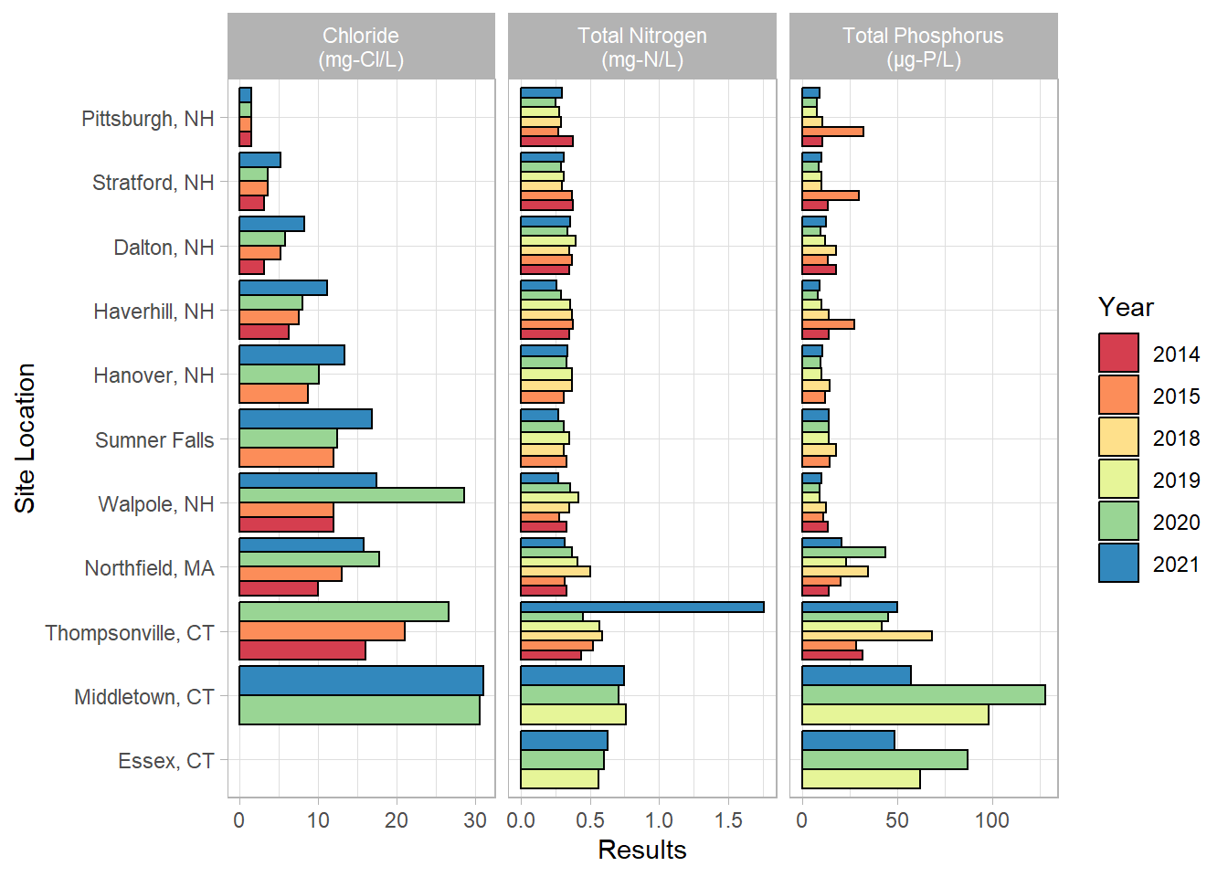
This is a look at all of the results from the mainstem sites over the years. As you can see, Connecticut was added later in the project life. In general, the concentrations increase from north to south, though they seem to peak at Middletown. Essex is brackish, so the chloride is omitted for that location since the water is naturally salty.
ggplot(tributary, aes(y = fct_reorder(SiteName, Lat), x = ResultValue, fill = Year)) +
  geom_col(color = "black", position = "dodge") +
  scale_fill_brewer(palette = "Spectral") +
  labs(x = "Results", y = "Site Location") +
  theme_light() +
  facet_grid(cols = vars(Parameter),
             rows = vars(EcoRegion),
             scales = "free",
             labeller = labeller(Parameter = parameter_labs, EcoRegion = label_both))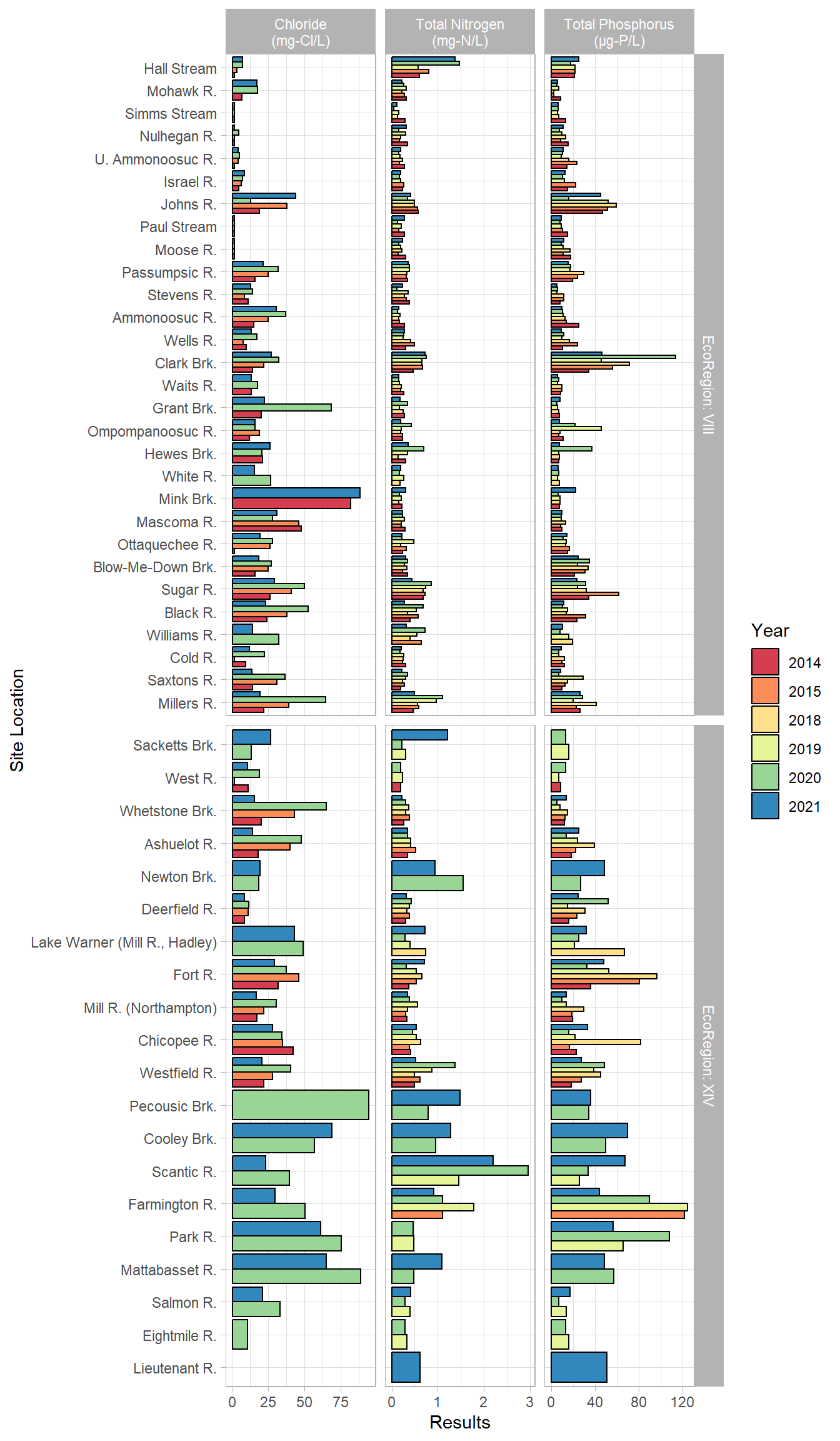
These are the results from all the tributaries, split up by EcoRegion and parameter. We expect to see higher nutrients in EcoRegion XIV than in VIII, which is demonstrated here. The tributaries are arranged from north to south again, but each tributary is affected also by how much urbanization and agriculture is within it, rather than its north-south orientation.
ggplot(tributary, aes(x = Est_loading, y = fct_reorder(SiteName, Drainage_sq_mi), fill = State)) +
  geom_bar(color = "black", stat = "summary", fun = "median") +
  scale_fill_brewer(palette = "Spectral") +
  labs(x = "Median Loading (lbs/day)", y = "Site Locations") +
  theme_light() +
  facet_grid(
    cols = vars(Parameter),
    rows = vars(EcoRegion),
    scales = "free",
    labeller = labeller(Parameter = loading_labs, EcoRegion = label_both))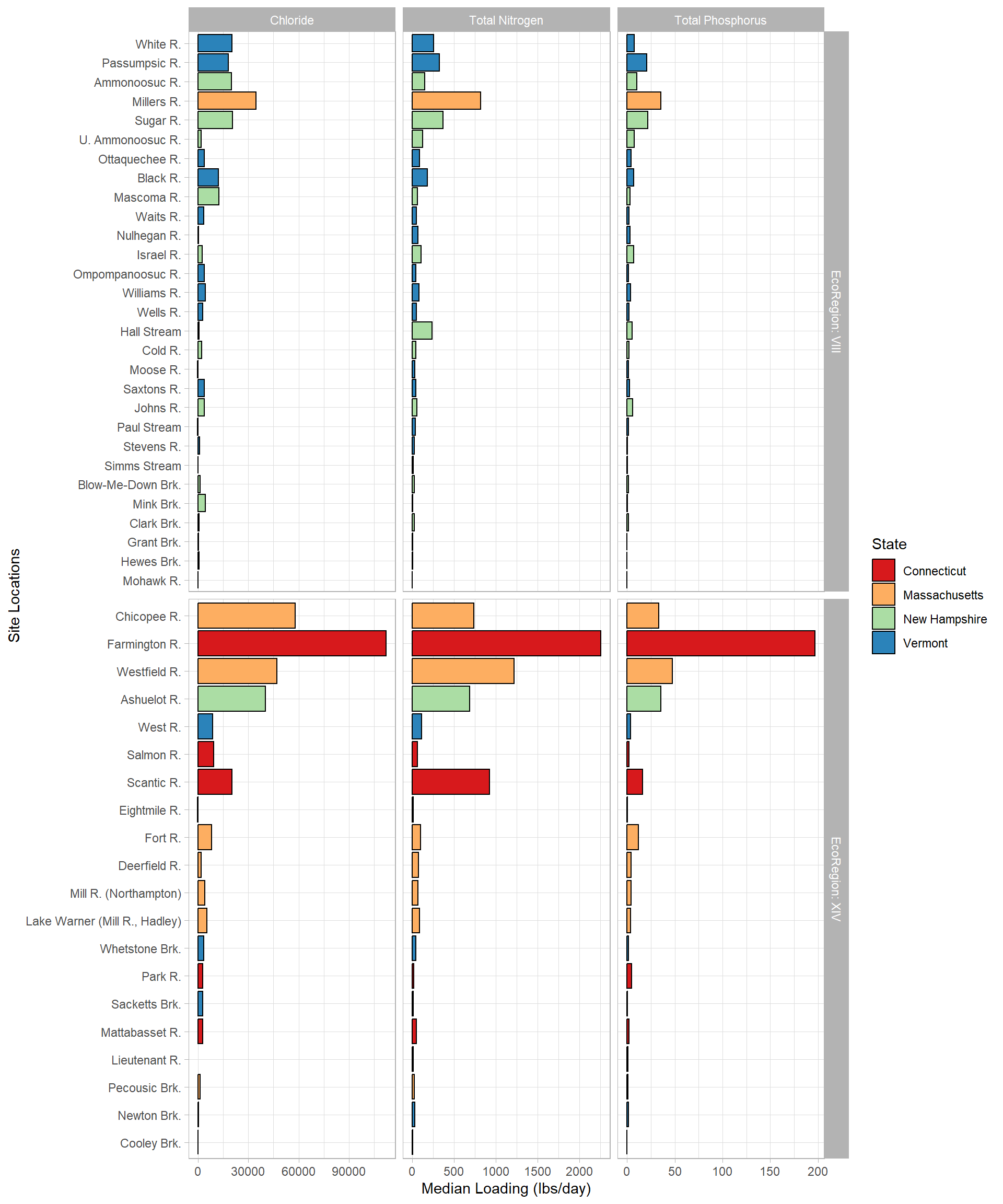
This graph has been very popular when I presented the results in 2019. I was easily able to also split it by EcoRegion using facet_grid(). If each tributary was contributing its “fair share” of chloride, nitrogen, and phosphorus, they would also (more or less) go from largest loading to smallest in each EcoRegion; we would also expect EcoRegion XIV. Some noteable over contributers are the Farmington, Millers, Scantic, and Fort Rivers.
ggplot(tributary, aes(y = Est_loading, x = ResultValue, color = State)) +
  geom_point() +
  scale_fill_brewer(palette = "Spectral") +
  labs(x = "Concentration", y = "Loading (lbs/day") +
  theme_light() +
  facet_wrap(vars(Parameter),
             scales = "free",
             labeller = labeller(Parameter = loading_labs))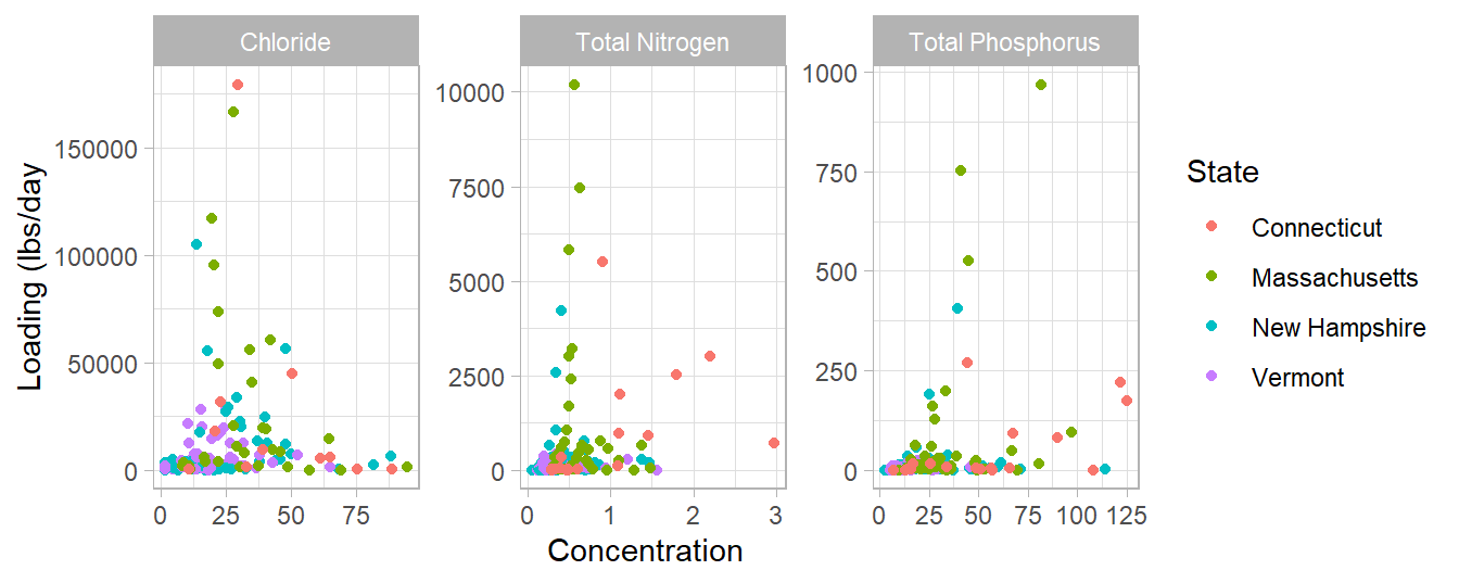
This graph shows the concentration versus the loading of each tributary sample. It is interesting that most of the sites contributing the highest loading of each parameter do not have the highest concentration, especially with chloride. If we wanted to direct restoration efforts on particular tributaries, those efforts should be targeted to watersheds that fall in the upper right quandrant of these graphs to have the biggest impact.
ggplot(tributary, aes(x = State, y = ResultValue, fill = Parameter)) +
  geom_violin() +
  scale_fill_brewer(palette = "Spectral") +
  theme_light() +
  guides(x = guide_axis(n.dodge = 2), fill = "none") +
  facet_grid(rows = vars(Parameter),
             cols = vars(EcoRegion),
             scales = "free",
             labeller = labeller(EcoRegion = label_both, Parameter = parameter_labs))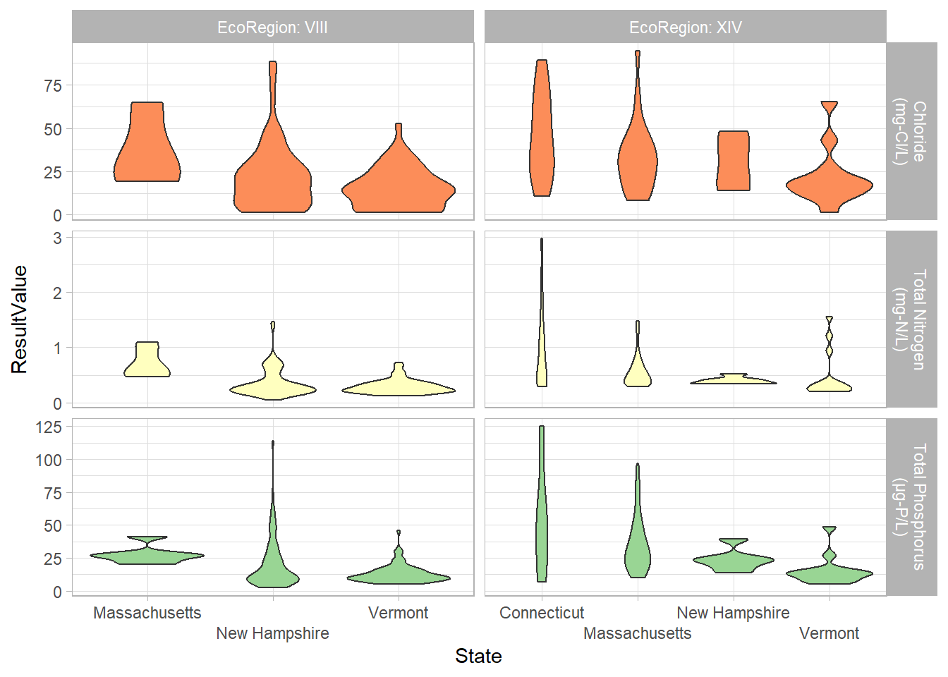
I was particularly interested in the utility of the violin plots. I have been criticized in the past by other professionals in my field for my reluctance to use box and whisker plots. Aside from the fact that they are nearly impossible to make in Excel, I have conducted some informal polls and found that non-scientists do not understand the information a box and whisker plot is trying to convey. These violin plots seem to present the distribution a little more intuitively. In this graph, we can see that Vermont and New Hampshire have bottom heavy plots (which is what we would like to see) and Connecticut and Massachusetts have more even distribution across the ranges of concentrations.
ggplot(tributary, aes(x = State, y = Est_loading, fill = Parameter)) +
  geom_violin() +
   scale_fill_brewer(palette = "Spectral") +
  labs(y = "Estimated Loading (lbs/day)") +
  theme_light() +
  guides(fill = "none") +
   facet_grid(rows = vars(Parameter),
              scales = "free",
              labeller = labeller(Parameter = loading_labs))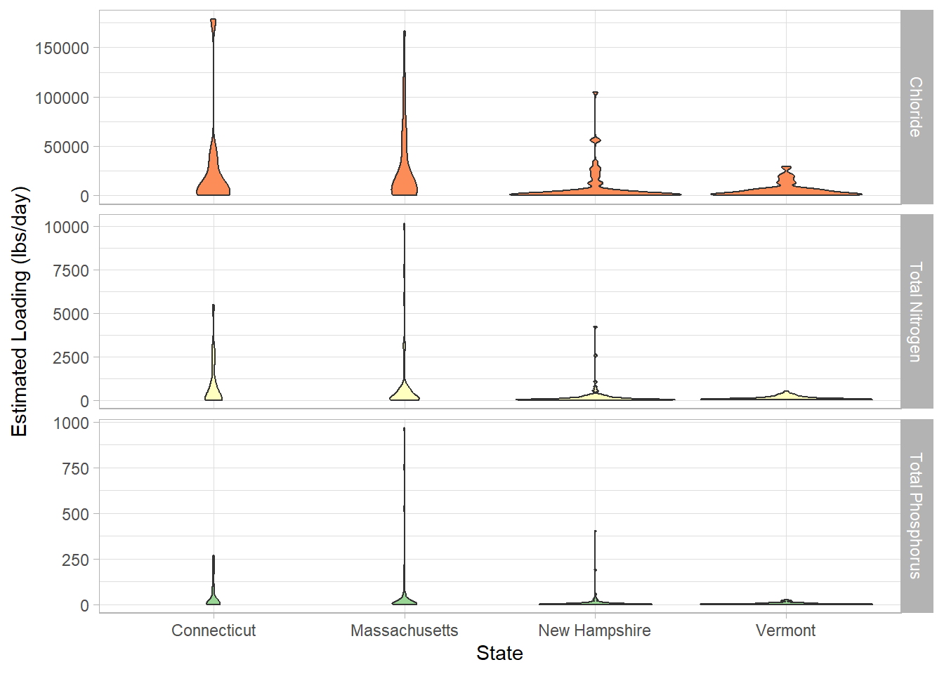
This is the same graph but looking at loading. Here, we can see that all the plots are bottom heavy with Connecticut and Massachusetts having the heavier hitting tributaries compared to New Hampshire and Vermont.
# Watershed States
watershed_states <- map_data("state") %>%
  filter(region %in% c("connecticut", "massachusetts", "vermont", "new hampshire")) %>%
           filter(!subregion %in% c("martha's vineyard", "nantucket"))
# map files
trib_map <- st_read("_data/maps/Splza_tribs.shp") %>%
  fortify() %>%
  mutate(SiteID = str_trim(SiteID))

mainstem_map <- st_read("_data/maps/Splza_main.shp") %>%
  fortify() %>%
  mutate(SiteID = str_trim(SiteID))

# join with data
trib_map_data <- splza_results_loading_no_outliers %>%
   filter(SiteType == "Tributary") %>%
  full_join(.,
  trib_map,
  by = c("SiteID" = "SiteID")) %>% #not sure why it made me do this, but just putting SiteID didn't work
    st_as_sf()

main_map_data <- splza_results_loading_no_outliers %>%
   filter(SiteType == "Mainstem") %>%
  full_join(.,
  mainstem_map,
  by = c("SiteID" = "SiteID")) %>%
    st_as_sf()
Making maps is also very important for presenting water quality data in a way that makes sense to the average viewer. I primarily present my work to the volunteers who collect the data, at public meetings, or to school children. The easier to understand, the better!
To set up these maps, I created a base of the four watershed states using the maps package, which I first did in Homework 3. I used the USGS StreamStats program and GIS to make a shapefile of all the tributaries and the mainstem sites that would be easy to join with the data in R. This map layer already existed prior to this project. I read this file in using the sf package and joined it with the data. Then the shapes were ready to be plotted in ggplot2.
filter(trib_map_data, Parameter == "TN") %>%
ggplot() +
  geom_polygon(data = watershed_states, aes(x = long, y = lat, group = region), color = "dark green", linetype = "dotted", fill="green", alpha=0.3) +
  expand_limits(x = watershed_states$long, y = watershed_states$lat) +
  scale_shape_identity() +
  coord_map() +
  geom_sf(aes(fill = ResultValue, color = Exceeds_criteria)) +
scale_fill_distiller(palette = "Blues", direction = 1, breaks = c(0, 0.4, 0.7, 1.5, 3), name = "Total Nitrogen\n(mg-N/L)") +
  scale_color_discrete(name = "EcoRegion Criteria") +
  theme_void() +
  facet_wrap(vars(Year))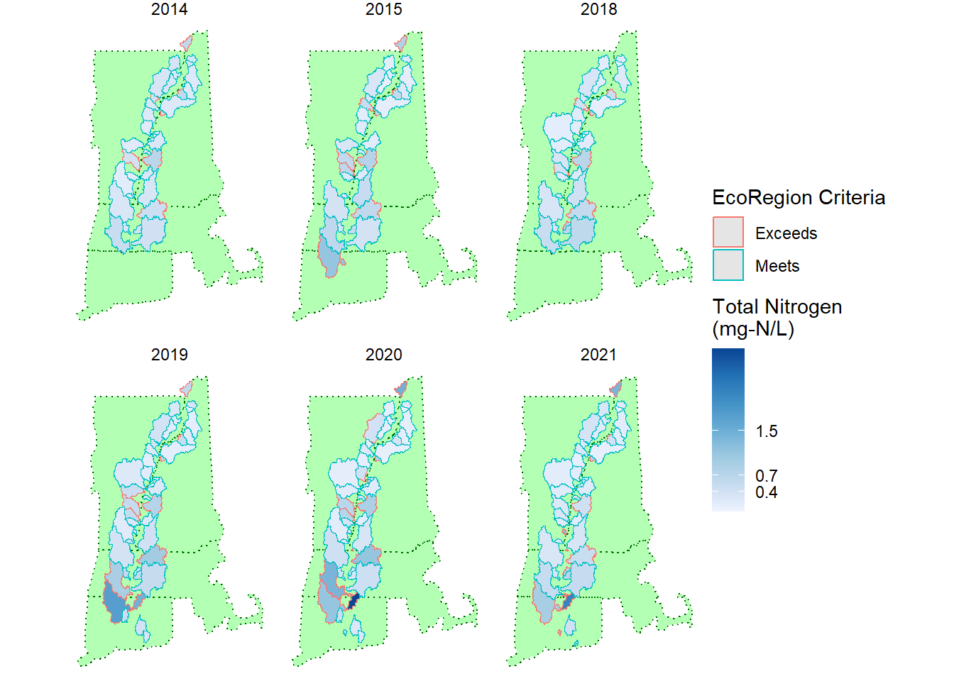
Using ggplot2 and facet_wrap() to create these maps is very useful. I used to have to make a different layer for each year in GIS and export it separately to put in my reports.
In this figure, you can see the relative concentrations and the outline indicates whether or not the watershed meets the criteria for its EcoRegion. It is particularly stark that only the Scantic River watershed is the darkest blue.
filter(main_map_data, Parameter == "TP") %>%
ggplot() +
  geom_polygon(data = watershed_states, aes(x = long, y = lat, group = region), color = "dark green", linetype = "dotted", fill="green", alpha=0.3) +
  expand_limits(x = watershed_states$long, y = watershed_states$lat) +
  scale_shape_identity() +
  coord_map() +
  geom_sf(aes(fill = ResultValue, color = Exceeds_criteria)) +
scale_fill_distiller(palette = "Reds", direction = 1, breaks = c(0, 10, 31, 60, 125), name = "Total Phosphorus\n(\u03bc/L)") +
  scale_color_discrete(name = "EcoRegion Criteria") +
  theme_void() +
  facet_wrap(vars(Year))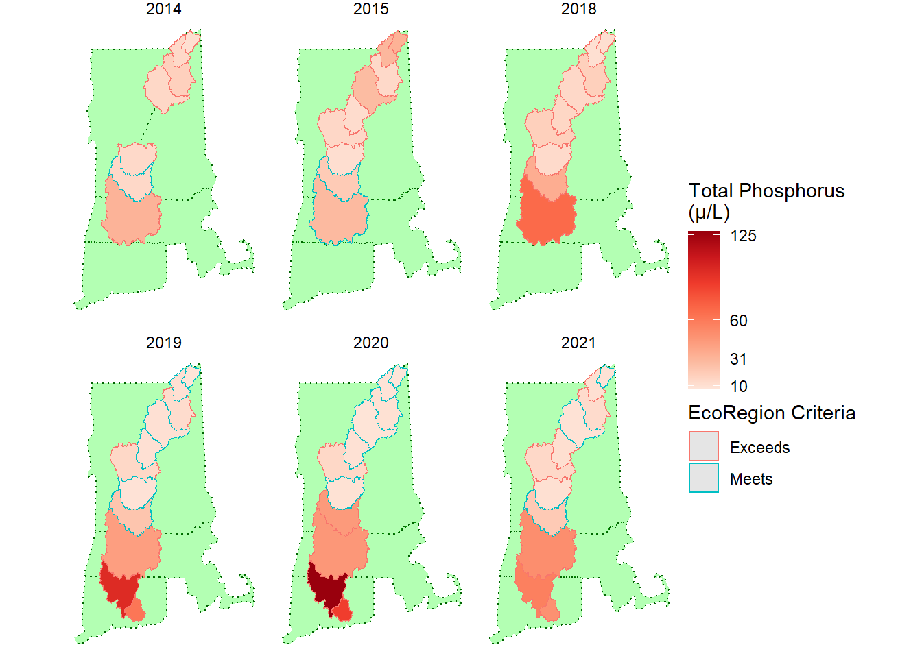
This is an example of a similar map with the mainstem sites instead of the tributaries.
filter(trib_map_data, Parameter == "Cl") %>%
  group_by(SiteName) %>%
  mutate("avg_yield" = mean(Est_yield)) %>%
ggplot() +
  geom_polygon(data = watershed_states, aes(x = long, y = lat, group = region), color = "dark green", linetype = "dotted", fill="green", alpha=0.3) +
  expand_limits(x = watershed_states$long, y = watershed_states$lat) +
  scale_shape_identity() +
  geom_sf(aes(fill = avg_yield)) +
  scale_fill_distiller(palette = "Purples", direction = 1, name = "Chloride\nAverage Yield\n(lbs/day/sq mi)") +
  theme_void()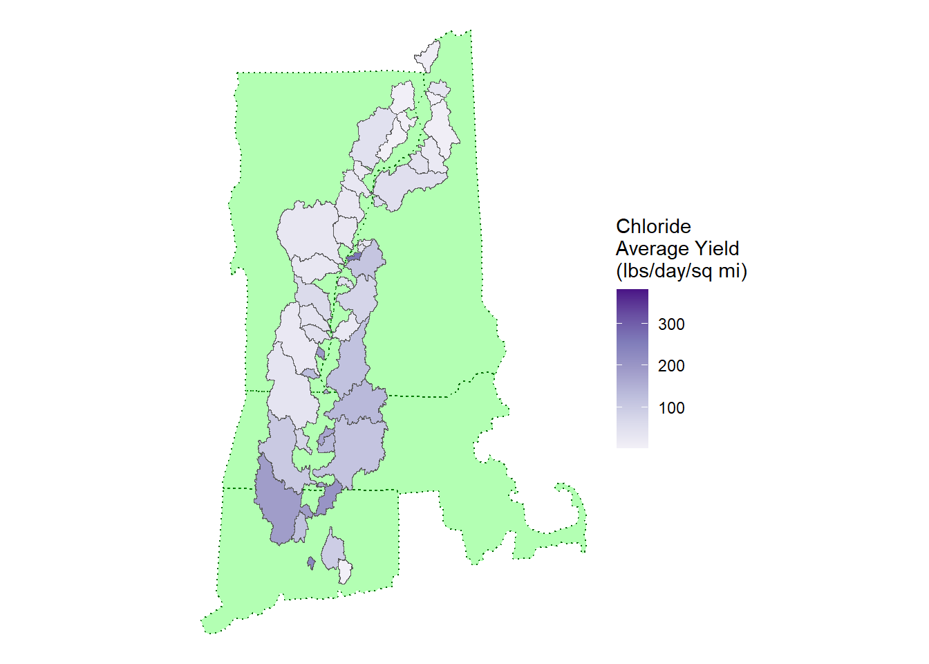
Finally, I made an example of the yields. The yields are the loading (lbs/day) adjusted for the area of the watershed. This helps adjust the concentrations to the impact of the watershed. Since the sizes of the watersheds are represented in the image, the yield is useful for mapping loading.
I chose to focus my project on practicing the visualizations I would need to create an effective report for work. I am expecting to be writing a report and following it up with an online presentation to all the partners who have participated in Samplepalooza over the years this winter. One of the challenges of the project has been communicating the results at a level acceptable to the state agencies that participate but presenting it in a way that is also understandable to the volunteers who collected samples. I think the ease with which I can now create maps (especially faceted by year) will make that task a lot easier.
Rebuilding the code to estimate the loading was the most difficult part of this project, but I learned a lot from it. I feel confident that I could build similar functions from scratch moving forward.
Rather than answering the specific question of what tributary is the biggest contributor of nitrogen or phosphorus, the research question is “Can I learn to use R to streamline how I work with my water quality data at work?” The answer is a resounding “Yes”!
There are lots of other water quality data that I work with constantly that are slightly different from the data I was working with here. The original loading calculation program that I was working with was highly specialized for Samplepalooza. By utilizing the principals of tidy data and using the new function with purrr, I am confident that I could use this same code to estimate loading for any water quality monitoring site that I work with.
As I was working on this project, I also identified the next few things I will do after the conclusion of this class. I will need to write a function to replace the data censored with a “<” or “>” with the appropriate value for statistical calculation. I will also need to write a function that can use the USGS gage data to classify flows as low, moderate, or high; this is based on the quartile that the flows fall in. Ideally, when presenting water quality data, only results from like flows should be compared. For example, the water quality conditions on a hot, dry summer day are expected to be significantly different than those during the spring snowmelt.
Dam Release Information. NAE Reservoir Regulation section. (2022). Retrieved December 17, 2022, from https://reservoircontrol.usace.army.mil/nae_ords/cwmsweb/cwms_web.cwmsweb.cwmsindex
De Cicco LA, Lorenz D, Hirsch RM, Watkins W, Johnson M (2022). dataRetrieval: R packages for discovering and retrieving water data available from U.S. federal hydrologic web services. doi:10.5066/P9X4L3GE, https://code.usgs.gov/water/dataRetrieval.
Drury, Travis. (2020) CT River 18-19 Sample Flow Estimates and Load Estimate Results.
Grolemund, G., & Wickham, H. (2016). R for Data Science: Import, Tidy, Transform, Visualize, and Model Data. O’Reilly Media.
U.S. Geological Survey, 2019, The StreamStats program, online at http://streamstats.usgs.gov
R Core Team. (2020). R: A language and environment for statistical computing. R Foundation for Statistical Computing, Vienna, Austria.https://www.r-project.org.
RStudio Team. (2019). RStudio: Integrated Development for R. RStudio, Inc., Boston, MA. https://www.rstudio.com.
Wickham H, Averick M, Bryan J, Chang W, McGowan LD, François R, Grolemund G, Hayes A, Henry L, Hester J, Kuhn M, Pedersen TL, Miller E, Bache SM, Müller K, Ooms J, Robinson D, Seidel DP, Spinu V, Takahashi K, Vaughan D, Wilke C, Woo K, Yutani H (2019). “Welcome to the tidyverse.” Journal of Open Source Software, 4(43), 1686. doi:10.21105/joss.01686 https://doi.org/10.21105/joss.01686.
```{r}
#Original loading code by volunteer:


########################################################################################
###   CT River 18-19 Sample Flow Estimates and Load Estimate Results               #####
###   Updated: 2020-03-19                                                          #####
###   Author: Travis Drury                                                         #####
###   Contact: .......................                                             #####
########################################################################################


########-------------------------------------------------------------------------#######
###       STEP 1: Set directory where all following data files are located           ###
########-------------------------------------------------------------------------#######

setwd("\\\\10.170.192.4/netshare/Education & Outreach/Water monitoring/Data Volunteer Work/Travis/Flow-weighted 18-19")


########--------------------------------------------------------------------------#######
###       STEP 2: Enter the name of the sampling results file                         ###
###       Must be a .CSV filetype and formatted the same as CT_18_19_results.csv      ###
###       Must have at least the following 5 columns:                                 ###
###       Date, SiteID, TN_mg_L, Nox_mg_L, TKN_calc_mg_L, TP_ug_L                     ###
########--------------------------------------------------------------------------#######

results.filename <- "CT_18_19_results.csv"


########--------------------------------------------------------------------------#######
###       STEP 3: Enter the name of the file with CRC Sampling Locations,             ###
###       CRC sampling location drainage areas, and USGS gages for each location      ###
###       Must be a CSV formatted the same as usgs_gages_for_sites.csv                ###
###       Must have at least the following 5 columns:                                 ###
###       SiteID, Drainage_sq_mi, Gage1, Gage2, USACOE_dam                            ###
########--------------------------------------------------------------------------#######

CRC_locations_gages <- "usgs_gage_for_sites.csv"


########--------------------------------------------------------------------------#######
###       STEP 4: Enter a name for the output CSV file                                ###
########--------------------------------------------------------------------------#######

output.name <- "CTRESULTS_2018_2019_EstimatedFlows_EstimatedLoads.csv"


########--------------------------------------------------------------------------#######
###       STEP 5: Run all code (including above) to estimate CRC sampling location    ###
###       flows and loads. If error presents which indicates flows are unavailable    ###
###       for a particular USGS gage, change gage in step 3 file and rerun all code   ###
########--------------------------------------------------------------------------#######


### ipak function used to install/load packages
ipak <- function(pkg){
  new.pkg <- pkg[!(pkg %in% installed.packages()[, "Package"])]
  if (length(new.pkg))
    install.packages(new.pkg, dependencies = TRUE, repos="http://cran.rstudio.com/", quiet = T, verbose = F)
  sapply(pkg, require, character.only = TRUE)
}
### Package List ####
packages <- c("tidyverse","dataRetrieval","measurements","dplyr","lubridate","bigrquery","rvest")
### Run the function
ipak(packages)

### Disables scientific notation
options(scipen=999)

### Bring in sampling results
ctresults <- read.csv(results.filename)

### Format date and create UniqueID
ctresults$Date <- as.Date(ctresults$Date,format="%m/%d/%Y")
ctresults$UniqueID <- paste0(ctresults$Date,"_",ctresults$SiteID)

### Bring in data on sampling locations (drainage area and USGS gages to use for flow estimation)
usgs_gages_for_sites <- read.csv(CRC_locations_gages)

### Add leading zero if dropped from gage numbers
usgs_gages_for_sites$Gage1[!is.na(usgs_gages_for_sites$Gage1)] <- paste0("0",usgs_gages_for_sites$Gage1[!is.na(usgs_gages_for_sites$Gage1)])
usgs_gages_for_sites$Gage2[!is.na(usgs_gages_for_sites$Gage2)] <- paste0("0",usgs_gages_for_sites$Gage2[!is.na(usgs_gages_for_sites$Gage2)])


### Match gages to data based on SiteID
ctresults_gages <- left_join(x=ctresults,y=usgs_gages_for_sites,by="SiteID")

### USGS mean daily discharge, first for Gage1, then for Gage2
for (i in 1:nrow(ctresults_gages)){
              if(!is.na(ctresults_gages$Gage1[i])){

                tempdv <- data.frame(readNWISdv(siteNumbers = ctresults_gages$Gage1[i], parameterCd = "00060",
                                                  startDate = ctresults_gages$Date[i],endDate = ctresults_gages$Date[i]))


                    if(nrow(tempdv) > 0){

                      ctresults_gages$Gage1_dv[i] <- as.numeric(as.character(tempdv[4]))

                      rm(tempdv)


                    } else {

                      rm(tempdv)
                       stop(paste0("No discharge data available at USGS gage ",ctresults_gages$Gage1[i], " on ",ctresults_gages$Date[i]," for sampling location ",ctresults_gages$SiteID[i],"."))
                    }

              } else {

                ctresults_gages$Gage1_dv[i] <- c("")

              }

}

for (i in 1:nrow(ctresults_gages)){
  if(!is.na(ctresults_gages$Gage2[i])){

    tempdv <- data.frame(readNWISdv(siteNumbers = ctresults_gages$Gage2[i], parameterCd = "00060",
                                    startDate = ctresults_gages$Date[i],endDate = ctresults_gages$Date[i]))


    if(nrow(tempdv) > 0){

      ctresults_gages$Gage2_dv[i] <- as.numeric(as.character(tempdv[4]))

      rm(tempdv)


    } else {

      rm(tempdv)
      stop(paste0("No discharge data available at USGS gage ",ctresults_gages$Gage2[i], " on ",ctresults_gages$Date[i]," for sampling location ",ctresults_gages$SiteID[i],"."))
    }

  } else {

    ctresults_gages$Gage2_dv[i] <- c("")

  }

}

### USGS gage drainage areas, first for Gage1 then for Gage2
for (i in 1:nrow(ctresults_gages)){
  if(!is.na(ctresults_gages$Gage1[i])){

    tempinfo <- data.frame(readNWISsite(siteNumbers = ctresults_gages$Gage1[i]))


    if(tempinfo[30] > 0){

      ctresults_gages$Gage1_area[i] <- as.numeric(as.character(tempinfo[30]))

      rm(tempinfo)


    } else {

      rm(tempinfo)
      stop(paste0("No watershed area data available for USGS gage ",ctresults_gages$Gage1[i], " for sampling location ",ctresults_gages$SiteID[i],"."))
    }

  } else {

    ctresults_gages$Gage1_area[i] <- c("")

  }

}

for (i in 1:nrow(ctresults_gages)){
  if(!is.na(ctresults_gages$Gage2[i])){

    tempinfo <- data.frame(readNWISsite(siteNumbers = ctresults_gages$Gage2[i]))


    if(tempinfo[30] > 0){

      ctresults_gages$Gage2_area[i] <- as.numeric(as.character(tempinfo[30]))

      rm(tempinfo)


    } else {

      rm(tempinfo)
      stop(paste0("No watershed area data available for USGS gage ",ctresults_gages$Gage2[i], " for sampling location ",ctresults_gages$SiteID[i],"."))
    }

  } else {

    ctresults_gages$Gage2_area[i] <- c("")

  }

}


### Calculate USGS gage csm (ft^3 per second per mi^2)
ctresults_gages$Gage1_dv <- as.numeric(as.character(ctresults_gages$Gage1_dv))
ctresults_gages$Gage1_area <- as.numeric(as.character(ctresults_gages$Gage1_area))
ctresults_gages$Gage2_dv <- as.numeric(as.character(ctresults_gages$Gage2_dv))
ctresults_gages$Gage2_area <- as.numeric(as.character(ctresults_gages$Gage2_area))

ctresults_gages <- ctresults_gages %>% mutate(Gage1_csm = Gage1_dv/Gage1_area,
                                              Gage2_csm = Gage2_dv/Gage2_area)


### Download Dam data for sites that use those flows

dam_data <- data.frame(matrix(ncol=3,nrow=0, dimnames=list(NULL, c("Date","Dam_code","dam_meandv"))))
unique_dates <- paste0(unique(ctresults_gages$Date))


for (i in unique_dates){

  url <- paste0("https://reservoircontrol.usace.army.mil/NE/pls/cwmsweb/cwms_web.apitable.xls?gagecode=UVD&days=1&enddate=",format.Date(i,"%m/%d/%Y"),"&interval_hrs=1")
  html_output <- read_html(url)
  html_tables <- html_nodes(html_output,"table")
  html_output_table <- html_table(html_tables[1],fill=TRUE,header=TRUE)
  html_table_df <- as.data.frame(html_output_table)
  temp_dam_data <- as.data.frame(matrix(ncol=3,nrow=2,c(i,i,"UVD_i","UVD_o",mean(as.numeric(as.character(html_table_df[1:24,6]))),mean(as.numeric(as.character(html_table_df[1:24,5]))))))
  colnames(temp_dam_data) <- c("Date","Dam_code","dam_meandv")
  dam_data <- dplyr::bind_rows(dam_data,temp_dam_data)
  rm(url,html_output,html_tables,html_output_table,html_table_df,temp_dam_data)

  url <- paste0("https://reservoircontrol.usace.army.mil/NE/pls/cwmsweb/cwms_web.apitable.xls?gagecode=NHD&days=1&enddate=",format.Date(i,"%m/%d/%Y"),"&interval_hrs=1")
  html_output <- read_html(url)
  html_tables <- html_nodes(html_output,"table")
  html_output_table <- html_table(html_tables[1],fill=TRUE,header=TRUE)
  html_table_df <- as.data.frame(html_output_table)
  temp_dam_data <- as.data.frame(matrix(ncol=3,nrow=2,c(i,i,"NHD_i","NHD_o",mean(as.numeric(as.character(html_table_df[1:24,6])),mean(as.numeric(as.character(html_table_df[1:24,5])))))))
  colnames(temp_dam_data) <- c("Date","Dam_code","dam_meandv")
  dam_data <- dplyr::bind_rows(dam_data,temp_dam_data)
  rm(url,html_output,html_tables,html_output_table,html_table_df,temp_dam_data)

  url <- paste0("https://reservoircontrol.usace.army.mil/NE/pls/cwmsweb/cwms_web.apitable.xls?gagecode=NSD&days=1&enddate=",format.Date(i,"%m/%d/%Y"),"&interval_hrs=1")
  html_output <- read_html(url)
  html_tables <- html_nodes(html_output,"table")
  html_output_table <- html_table(html_tables[1],fill=TRUE,header=TRUE)
  html_table_df <- as.data.frame(html_output_table)
  temp_dam_data <- as.data.frame(matrix(ncol=3,nrow=2,c(i,i,"NSD_i","NSD_o",mean(as.numeric(as.character(html_table_df[1:24,6])),mean(as.numeric(as.character(html_table_df[1:24,5])))))))
  colnames(temp_dam_data) <- c("Date","Dam_code","dam_meandv")
  dam_data <- dplyr::bind_rows(dam_data,temp_dam_data)
  rm(url,html_output,html_tables,html_output_table,html_table_df,temp_dam_data)

  }

### Add drainage area of dams

dam_data <- dam_data %>% mutate(dam_area = case_when(Dam_code=="UVD_i" ~ 126,
                                                     Dam_code=="UVD_o" ~ 126,
                                                     Dam_code=="NHD_i" ~ 220,
                                                     Dam_code=="NHD_o" ~ 220,
                                                     Dam_code=="NSD_i" ~ 158,
                                                     Dam_code=="NSD_o" ~ 158))

### Add csm for dam inflow and outflow (ft^3 per second per mi^2)

dam_data$dam_meandv <- as.numeric(as.character(dam_data$dam_meandv))
dam_data$Date <- as.Date(dam_data$Date,format="%Y-%m-%d")

dam_data <- dam_data %>% mutate(dam_csm = dam_meandv/dam_area)


### Add dam data to results
ctresults_gages <- left_join(x=ctresults_gages,y=dam_data,by=c("USACOE_dam"="Dam_code","Date"="Date"))

### Calculate estimated flows in cfs, 25-CNT has special calculation
ctresults_gages <- ctresults_gages %>% mutate(Est_dv_cfs = case_when(!is.na(dam_csm) ~ dam_csm*Drainage_sq_mi,
                                                                      !is.na(Gage1_csm) & !is.na(Gage2_csm) & SiteID != "25-CNT" ~ ((Gage1_csm+Gage2_csm)/2)*Drainage_sq_mi,
                                                                      !is.na(Gage1_csm) & is.na(Gage2_csm) & SiteID != "25-CNT" ~ Gage1_csm*Drainage_sq_mi,
                                                                      !is.na(Gage1_csm) & SiteID == "25-CNT" ~ (Gage2_csm*221) + (Gage1_csm*(Drainage_sq_mi - 221))))


### Calculate loading
### Note: 5.393771 and 0.005394 are calculated conversion factors to result in pounds/day

### mg_L_conversion_factor = mg/L * ft3/second * 28.3168 L/1 ft3 * 1 lb/453592 mg * 86400 second/1 day
### ug_L_conversion_factor = mg/L * ft3/second * 28.3168 L/1 ft3 * 1 lb/453592370 ug * 86400 second/1 day

mg_L_conversion_factor <- 5.393771
ug_L_conversion_factor <- 0.005394


### ADD CODE TO CHANGE LESS THANS TO ZERO

#Replace "less than" values with zero
for (i in 1:nrow(ctresults_gages)){
  if(grepl("<",ctresults_gages$TN_mg_L[i],fixed=FALSE)){
    ctresults_gages$TN_mg_L[i] <- 0
  }}

for (i in 1:nrow(ctresults_gages)){
  if(grepl("<",ctresults_gages$Nox_mg_L[i],fixed=FALSE)){
    ctresults_gages$Nox_mg_L[i] <- 0
  }}

for (i in 1:nrow(ctresults_gages)){
  if(grepl("<",ctresults_gages$TKN_calc_mg_L[i],fixed=FALSE)){
    ctresults_gages$TKN_calc_mg_L[i] <- 0
  }}

for (i in 1:nrow(ctresults_gages)){
  if(grepl("<",ctresults_gages$TP_ug_L[i],fixed=FALSE)){
    ctresults_gages$TP_ug_L[i] <- 0
  }}

ctresults_gages$TN_mg_L <- as.numeric(as.character(ctresults_gages$TN_mg_L))
ctresults_gages$Nox_mg_L <- as.numeric(as.character(ctresults_gages$Nox_mg_L))
ctresults_gages$TKN_calc_mg_L <- as.numeric(as.character(ctresults_gages$TKN_calc_mg_L))
ctresults_gages$TP_ug_L <- as.numeric(as.character(ctresults_gages$TP_ug_L))

ctresults_gages <-  ctresults_gages %>% mutate(TN_lb_day = TN_mg_L*Est_dv_cfs*mg_L_conversion_factor,
                                               Nox_lb_day = Nox_mg_L*Est_dv_cfs*mg_L_conversion_factor,
                                               TKN_lb_day = TKN_calc_mg_L*Est_dv_cfs*mg_L_conversion_factor,
                                               TP_lb_day = TP_ug_L*Est_dv_cfs*ug_L_conversion_factor)


### Export data

ctresults_output <- ctresults_gages %>% select(Date, SiteID, Name, TN_mg_L, Nox_mg_L, TKN_calc_mg_L, TP_ug_L, Est_dv_cfs, TN_lb_day, Nox_lb_day, TKN_lb_day, TP_lb_day)

write.csv(ctresults_output,output.name)
```