    County               Year      Homeless (Count)   Population
 Length:201         Min.   :2018   Min.   :   0.0   Min.   :   8367
 Class :character   1st Qu.:2018   1st Qu.:  11.0   1st Qu.:  28089
 Mode  :character   Median :2019   Median : 151.0   Median : 130642
                    Mean   :2019   Mean   : 427.8   Mean   : 317746
                    3rd Qu.:2020   3rd Qu.: 563.0   3rd Qu.: 367471
                    Max.   :2020   Max.   :3516.0   Max.   :2864600

 Unemployment Rate   Median Inc    Incarceration (Rateper1000) Poverty (Count)
 Min.   : 2.100    Min.   :34583   Min.   : 0.60               Min.   :   906
 1st Qu.: 3.400    1st Qu.:41401   1st Qu.: 2.50               1st Qu.:  4901
 Median : 4.000    Median :50640   Median : 3.40               Median : 16210
 Mean   : 4.697    Mean   :51116   Mean   : 3.84               Mean   : 42922
 3rd Qu.: 5.600    3rd Qu.:58093   3rd Qu.: 4.50               3rd Qu.: 46034
 Max.   :13.500    Max.   :83803   Max.   :18.60               Max.   :482656

 Drug Arrests (Count) Relocated (Rate) Sub Abuse Enrollment (Count)
 Min.   :   13        Min.   : 4.689   Min.   :   5.0
 1st Qu.:  225        1st Qu.:11.244   1st Qu.:  76.0
 Median :  729        Median :12.700   Median : 250.0
 Mean   : 1558        Mean   :13.288   Mean   : 877.6
 3rd Qu.: 1903        3rd Qu.:14.544   3rd Qu.:1030.0
 Max.   :13038        Max.   :22.553   Max.   :6272.0

 Adult Psych Beds (Count) Severe Housing Problems (Rate) Forcible Sex (Count)
 Min.   :  0.00           Min.   : 9.6                   Min.   :   0.0
 1st Qu.:  0.00           1st Qu.:13.3                   1st Qu.:  14.0
 Median :  0.00           Median :15.4                   Median :  45.0
 Mean   : 66.26           Mean   :15.8                   Mean   : 170.5
 3rd Qu.: 84.00           3rd Qu.:17.3                   3rd Qu.: 225.0
 Max.   :778.00           Max.   :29.8                   Max.   :1408.0
                          NA's   :134
 Foster Care (Count)
 Min.   :   3.0
 1st Qu.:  33.0
 Median : 153.0
 Mean   : 326.1
 3rd Qu.: 353.0
 Max.   :2289.0
DACSS 601: Florida Homelessness
Quantitative Review by County
finalproject
shelton
homelessness
Homelessness in Florida
florida_1820.csv contains population figures, homelessness counts, poverty counts and other demographic indicators3 at the county level from 2018 to 2020. All 67 Florida counties have data for the 3 years, resulting in 201 observations of 15 variables. Each observation provides a count (or rate) for all variables from a single county for a year. The variables selected closely mirror the stressors mentioned in the reference study (Zugazaga), along with supplementary variables in an attempt to completely capture the circumstances.
Homelessness is a complex living situation with several qualifying conditions; at its simplest state, the U.S Dept. of Housing and Urban Development defines it as lacking a fixed, regular nighttime residence (not a shelter) or having a nighttime residence not designed for human accommodation1.
On a single night in 2020, over 500,0002 people experienced homelessness in the United States. Florida - the third largest state by population - had the fourth largest homeless population of 2020 with 27,4872.
Florida counties represent a wide range of demographic profiles; the state is a hub to a variety of industries including tourism, defense, agriculture, and information technology. Investigating homelessness in Florida counties with robust data can lead to several conclusions about who is being impacted where, and how state policy is failing (or aiding) groups of a diverse population.
Introduction
Carole Zugazaga’s 2004 study of 54 single homeless men, 54 single homeless women, and 54 homeless women with children in the Central Florida area investigated stressful life events common among homeless people. Interview responses revealed that women were more likely to have been sexually or physically assaulted, while men were more likely to have been incarcerated or abuse drugs/alcohol. Homeless women with children were more likely to be in foster care as a youth.
Nearly a decade later, county-level data can be used to investigate the relationship between Zugazaga’s reported stressful life events (incarceration, drug arrests, poverty, forcible sex, foster care)3 and homelessness rates.
Homelessness is not a new issue in the United States, yet homeless policy targets elimination via criminalization rather than prevention. A 2019 article from Homeless Voice provides a brief description of homeless policy in major citites across Florida. Despite state and federal governments being aware of the circumstances that increase vulnerability to homelessness for decades, I anticipate at least one Zugazaga’s five stressors to remain significant in a model relating stressors to Florida homelessness counts 2018-2020.
The data were collected from the Florida Department of Health. Variable names3 were used as search indicators to produce counts for Florida counties. Unfortunately, we cannot accurately analyze the effect of COVID-19 as data is incomplete for the majority of counties in 2021.
Read in and tidying were done in a separate file. The process began as laborious, but was lightened by the discovery of 10 year tables. Before this discovery, I would enter a variable name into the search bar of Florida Department of Health, select 2018, and download the .xlsx file to my personal data folder. readxl was used to bring in the file, and mutate created a date column filled with 2018. Once the data was appropriate, I saved it in the environment under variable2018. This was repeated for years 2019 and 2020. Then all three tibbles were full _join by County to provide a dataset with 201 observations (67 counties by 3 years) and three variables, County, Year, and the variable measurement itself . This was written as a .csv back to the same personal data folder.

Once learning that I could draw 10-year tables from the website rather than having to download three individual .xlsx files, the process became smoother. Now, I would only rename excess years as “delete” to get a table of measurements for only 2018, 2019, and 2020. pivot_longer then moved the years to a self-titled column and transferred the values to a column of my naming. This was written as a .csv.

I then merged all the tables and wrote this as a .csv florida_full. I completed a sanity check using distinct county names to ensure I had 201 observations of 15 variables as desired.


Expanding Intro to Data exposes summary statistics including mean, range, quantiles, and standard deviation for all 15 variables. The table below the summaries provides arranged figures for basic parameters of interest grouped by county. The data was nearly tidy, with complete observations for each variable aside from one - Severe Housing Issues rates for 2019 and 2020 (unrecorded) - these are later filled in with 2018’s value for the regression analysis.
Visualizations and Analysis
ggplot2 is used to visualize important relationships between homeless counts and Zugazaga’s stressors. The Florida counties have been categorized into 4 Regions and 3 Income Levels:

Code
# Categorize by regions... conditional better perhaps?


florida_og_plot <- florida_og_rates %>%
                    mutate('Region' = case_when(County == 'Escambia' |
                                              County == 'Santa Rosa'|
                                              County == 'Okaloosa'|
                                              County == 'Walton'|
                                              County == 'Holmes'|
                                              County == 'Washington'|
                                              County == 'Bay'|
                                              County == 'Jackson'|
                                              County == 'Calhoun'|
                                              County == 'Gulf'|
                                              County == 'Gadsden'|
                                              County == 'Escambia'|
                                              County == 'Liberty'|
                                              County == 'Leon'|
                                              County == 'Wakulla'|
                                              County == 'Franklin' |
                                              County == 'Jefferson'|
                                              County == 'Madison'|
                                              County == 'Taylor' ~
'Northwest',
                                              County == 'Hamilton'|
                                              County == 'Suwannee'|
                                              County == 'Lafayette'|
                                              County == 'Dixie'|
                                              County == 'Gilchrist'|
                                              County == 'Union'|
                                              County == 'Baker'|
                                              County == 'Columbia'|
                                              County == 'Nassau'|
                                              County == 'Levy'|
                                              County == 'Bradford'|
                                              County == 'Alachua'|
                                              County == 'Nassau'|
                                              County == 'Duval'|
                                              County == 'Putnam'|
                                              County == 'Marion'|
                                              County == 'Volusia'|
                                              County == 'Flagler'|
                                              County == 'Citrus'|
                                              County == 'Clay'|
                                              County == 'St. Johns' ~
'North',
                                              County == 'Lake'|
                                              County == 'Sumter'|
                                              County == 'Seminole'|
                                              County == 'Orange'|
                                              County == 'Hernando'|
                                              County == 'Pasco'|
                                              County == 'Brevard'|
                                              County == 'Indian River'|
                                              County == 'Pinellas'|
                                              County == 'Hillsborough'|
                                              County == 'Polk'|
                                              County == 'Osceola'|
                                              County == 'Hardee'|
                                              County == 'Manatee'|
                                              County == 'Okeechobee'|
                                              County == 'Highlands' ~
'Central',
                                              County == 'St. Lucie'|
                                              County == 'Sarasota'|
                                              County == 'Martin'|
                                              County == 'Palm Beach'|
                                              County == 'Collier'|
                                              County == 'Broward'|
                                              County == 'Lee'|
                                              County == 'DeSoto'|
                                              County == 'Charlotte'|
                                              County == 'Hendry'|
                                              County == 'Monroe'|
                                              County == 'Miami-Dade'|
                                              County == 'Glades'|
                                              County == 'Hendry'
~ 'South'))

# Categorize by Median Income Level

florida_og_plot <- florida_og_plot %>%
                    mutate('Income Level' = case_when(
                    `Median Inc` >= 60000 ~ 'High',
                    `Median Inc` < 60000 &
                    `Median Inc` >= 40000 ~ 'Medium',
                    `Median Inc` < 40000 ~ 'Low'))
b) Homeless Rate by Region
Code
# Plot 2

florida_box <- florida_og_plot %>%
    mutate(`Homeless (Rate)` = `Homeless (Rate)`*100 )%>%
      mutate(`Region`=fct_relevel(`Region`, "Northwest", "North", "Central", "South"))%>%
      ggplot(aes(y=`Homeless (Rate)`, x=`Region`, fill=`Region`)) +
        geom_boxplot(alpha=0.7)+
  #Scale of y axis
          scale_y_continuous(breaks=(seq(0,1.5,by=.25)))+
  # Dimensions of graph
            coord_cartesian(ylim=c(0,1.5)) +
              coord_flip()+
                scale_fill_brewer(palette = 'Set2')+
                                   theme_grey()+
                                     theme(legend.position = "none")+
                                        labs(title= "Florida Homeless Rates",
                                             subtitle="2018-2020",
                                              x= " ",
                                                y= "Homeless Rate (%)",
                                            caption = "Visualized by Region")

florida_box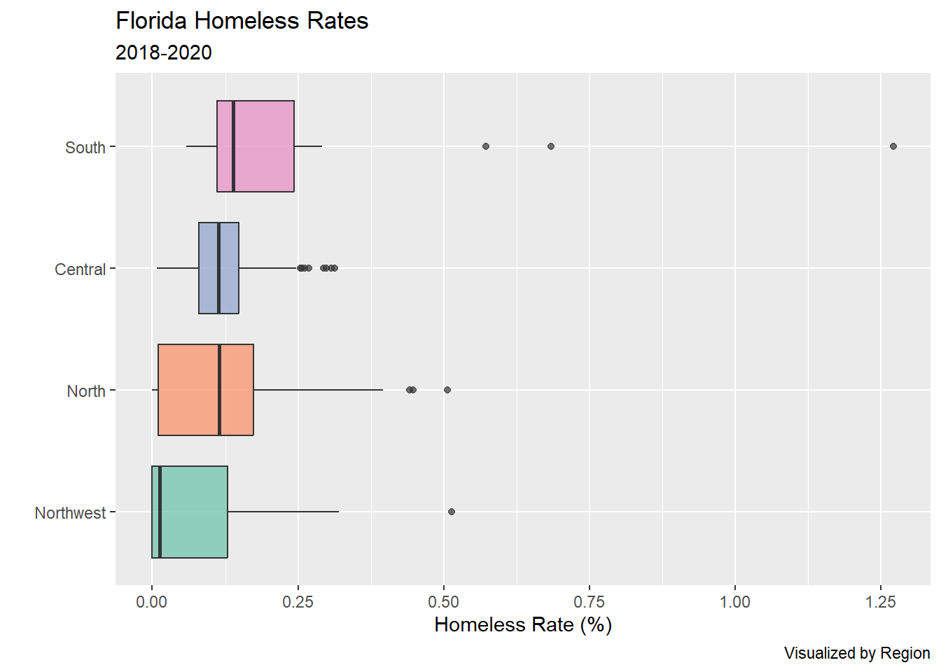
A look at the distributions of homeless rates across Florida counties displays where the highest rates in the state exists.
The state is generally uniform, with the bulk of each region’s distribution sitting below 0.25% of county populations.
The largest difference is between the distributions of Northwest Florida and South Florida. This can be attributed to the stark contrast in where the population in these regions are living.
South Florida is the most urbanized region in the state, with millions living in Miami, Ft. Lauderdale, and West Palm Beach; Northwest Florida is quite the opposite, with small coastal towns and rural inland towns reminiscent of Southern Alabama or Georgia.
c) Homeless Rate by Income Level
Code
# Plot 3
#Relevel Income, Mutate Response
florida_income <- florida_og_plot %>%
    mutate(`Homeless (Rate)` = `Homeless (Rate)`*100)%>%
      mutate(`Income Level` = fct_relevel(`Income Level`, "Low", "Medium", "High"))%>%
      ggplot(aes(y=`Homeless (Rate)`, x=`Region`,
                  fill=`Income Level`,
                    )) +
      geom_bar(position='dodge', stat='identity')+

              scale_fill_brewer(palette = 'Set2')+
                                   theme_grey()+

                    labs(title= "Barplot: Income Level x Homeless Rate",
                           subtitle="2018-2020",
                              x= "Region",
                                y= "Homeless Rate (%)",
                                  caption = "Visualized by Income Level")

florida_income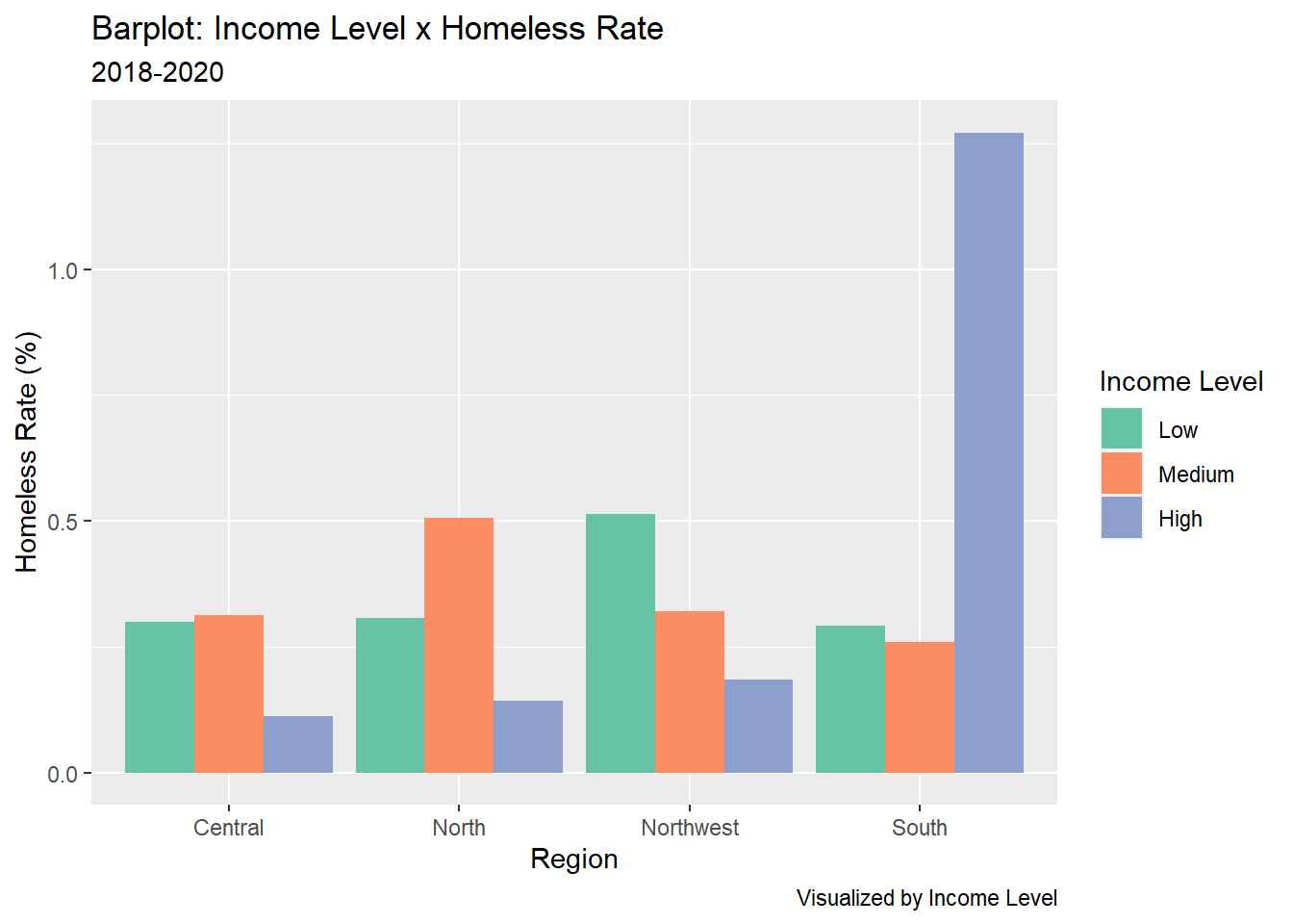
The barplot further details the differences mentioned in
Plot 2. Regions where the populations are less urbanized show Low Income counties reflecting a higher homeless rate as one would assume.Once entering South Florida, wealth disparities in urbanized areas breaks this trend -counties with high income now report high homeless rates
d) Homeless Rate x Incarceration Rate per1000
Code
#Plot 4

florida_incarc <- florida_og_plot %>%
    mutate(`Homeless (Rate)` = `Homeless (Rate)`*100,
           `Incarceration (Rateper1000)`= `Incarceration (Rateper1000)`/10)%>%
      ggplot(aes(y=`Homeless (Rate)`,
                  x=`Incarceration (Rateper1000)`,
                    color=`Region`,
                      label=`County`)) +
      geom_point(alpha=0.7)+
  # Must include because of label aesthetic
      ggrepel::geom_text_repel(show.legend = FALSE,
                  max.overlaps = 15,
                  alpha=0.7,
                    size=2.5,
                      nudge_x = -.05,
                        nudge_y =.05)+

              scale_fill_brewer(palette = 'Set2')+
                                   theme_grey()+
              # Titles, Axes, Caption
                    labs(title= "Scatterplot: Incarceration x Homeless Rate",
                           subtitle="2018-2020",
                              x= "Incarceration Rate (per100)",
                                y= "Homeless Rate (%)",
                                  caption = "Visualized by Region")

florida_incarc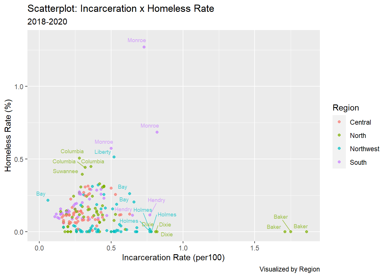
One of Zugazaga’s male stressors
Incarceration Rateis illustrated with Homeless Rate; a positive trend exists relating incarceration rates and homelessness rates across Florida counties.- Many state correctional facilities are located in rural counties, explaining both Baker and Monroe observations’ large influence on the plot.
e) Homeless Rate x Drug Arrest Rate
Code
#Plot 4

florida_drug <- florida_og_plot %>%
    mutate(`Homeless (Rate)` = `Homeless (Rate)`*100,
           `Drug Arrests (Rate)`= `Drug Arrests (Rate)`*100)%>%
      ggplot(aes(y=`Homeless (Rate)`,
                  x=`Drug Arrests (Rate)`,
                    color=`Region`,
                      label=`County`)) +
      geom_point(alpha=0.7)+
  # Must include because of label aesthetic
      ggrepel::geom_text_repel(show.legend = FALSE,
                  max.overlaps = 15,
                  alpha=0.7,
                    size=2.5,
                      nudge_x = -.05,
                        nudge_y =.05)+

              scale_fill_brewer(palette = 'Set2')+
                                   theme_grey()+

                    labs(title= "Scatterplot: Drug Arrest Rate x Homeless Rate",
                           subtitle="2018-2020",
                              x= "Drug Arrests (Rate)",
                                y= "Homeless Rate (%)",
                                  caption = "Visualized by Region")

florida_drug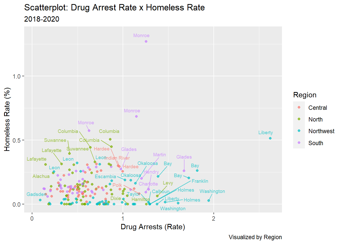
A similar positive association is seen comparing the homeless rate of a county with its
Drug Arrest (Rate).- The high influence of Northwest Florida is likely due to stricter drug policies held by police in less urbanized areas.
on Assumption of Validity
While over 10 variables are predicting Homeless (Rate) across Florida counties, there are still limitations when attempting to comment on the magnitude of an individual stressor. Stressors influence homelessness by driving those in severe situations out of their home or away from their place of origin. Homeless (Rate) is not an ideal measure of magnitude as the homeless population migrating to escape or avoid certain stressors would result in counties with low stressor values having a higher homeless population; this effect is left unexplained by the following models.
The variable
Relocated (Rate)is included as an attempt to control for new movement, however this doesn’t completely capture county-to-county migration.FL Charts has data that records Population Who Lived in a Different County One Year Earlier, however with the data spanning 2009-2014, using values recorded 4 years prior to our data isn’t desirable either.
The most appropriate data to accurately capture county-to-county migration is here via the US Census Bureau. The
-In, -Out, -Net...spreadsheet provides totals for each county in the United States and movement to all other US counties; unfortunately, this data is too complex to wrangle into the simple data setflorida_1820.csv.
on Assumption of Linearity
Code
# Fit 1: A Linear Regression Model With All Vars

# Checking Linearity of variables not supported by our literature
# Correlation Matrix
florida_matrix <- florida_og_rates %>%
                    select(-c(contains("Count"),
                              'Year',
                              'Poverty (Rate)',
                              'Severe Housing Problems (Rate)',
                              'Incarceration (Rateper1000)',
                              'Sub Abuse Enrollment (Rate)',
                              'Drug Arrests (Rate)',
                              'Adult Psych Beds (Rate)',
                              'Foster Care (Rate)',
                              'Forcible Sex (Rate)' ))%>%
                      pairs()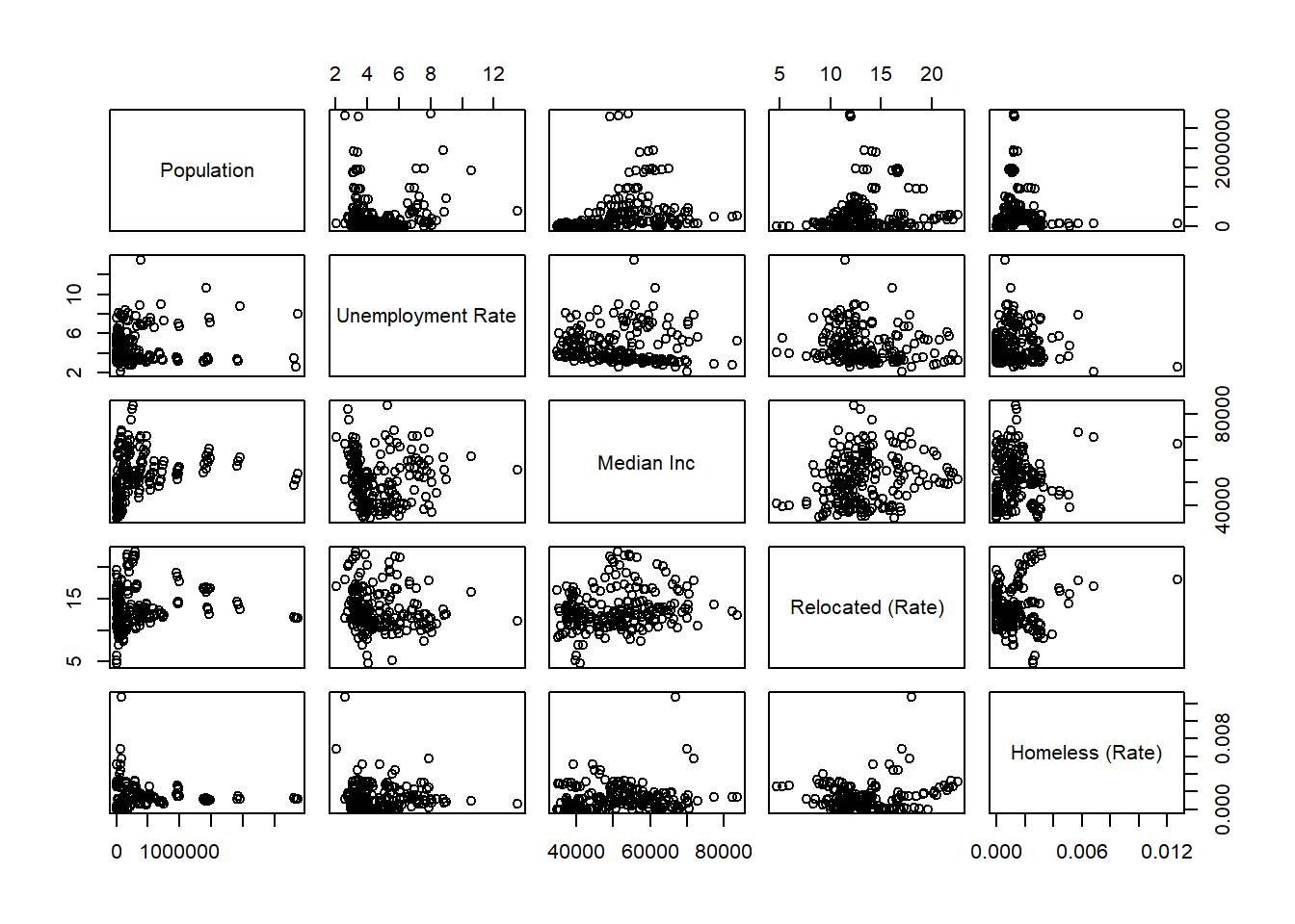
Code
florida_matrixNULLA quick look at stressors with a relationship to homelessness not mentioned in Zugazaga’s study, or those that needed further investigation are shown here to confirm linearity with the response, Homeless (Rate). Checking the bottom row,the associations are weak, but a linear approximation is appropriate.
Linear Regression Models
Fit 1: Diagnostics
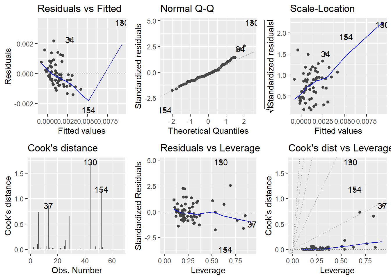
Fit 1does a poor job of obeying the assumptions regarding residuals of linear regression.Residuals vs Fittedshows a negative trend the greater the fitted value is, violating the linearity and independence assumption.Scale - Locationconfirms this as the standardized residuals increase in magnitude the greater the fitted value is.
Q-Q Plotshows a deviation from the diagonal, violating the assumption that residuals follow an approximately Normal distributionThere are several points that could be considered outliers due to their residual or leverage value, how greatly they influence the points around them in the model.
Monroe County (130), Hardee County (73), and Columbia County (34) all have large positive residuals, indicating our model greatly under-estimated the number of homeless people in this county.
Baker County (4) has worryingly high leverage, its explanatory values have great influence on the data
All of these outliers represent sparsely populated, rural counties, typically outside of more urbanized areas; hence large values for stressors will command great influence on the model.
Fit 2: Diagnostics
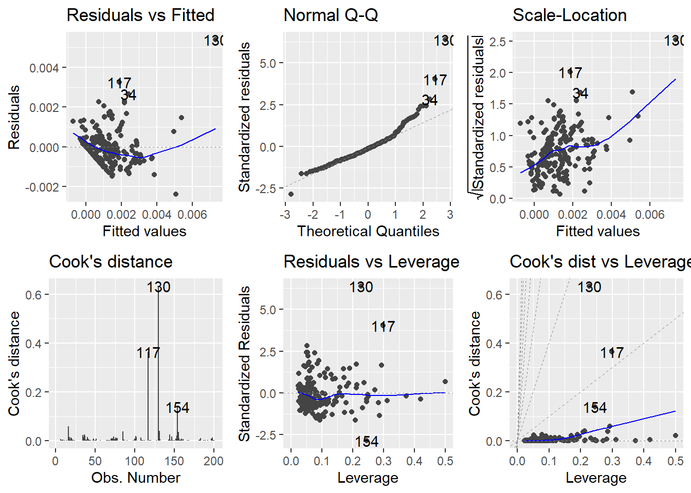
Using all observations in
Fit 2has not improved the diagnostic plots, but including 2019 and 2020 values has revealed new outliers.2020 produced Liberty County (117) as an outlier, a small, rural county in the Panhandle of Florida.
In late 2018, Hurricane Michael devastated the area; the influence of this observation is likely a direct result of measurements being altered greatly or even unaccounted during 2019 due to the population being “in a transitional state”
Liberty’s records in 2020 will show a vast difference to the incomplete measures of 2019
Model Selection
- Comparing Residuals Sum Squared and R2
Fit 2,Fit 3, andFit 4I would select Fit 3 for inference. AlthoughFit 4(with lag) had a lower Residual Sum Squared value, I appreciate the completeness ofFit 3and believe the extra variables provide a better picture of how stressors impact the homeless population in Florida.
Transforming the data into panel data produces more accurate coefficients, as rather than 201 individual observations, the model considers 3 years of 67 individual observations. This results in smaller standard error. The R^2 is only considered in passing, as the goal of the study is inference not prediction.
Research Question:
All of Zugazaga’s effects had plausible signs demonstrating their influence on homelessness in
Fit 3, but onlyDrug Arrests (Rate)was significant at the0.05level as hypothesized. This significance is a comment on the mathematical properties of the model rather than on the real-life effect of the stressors, which all are influential situations that can contribute to homelessness.Drug Arrests (Rate)positive slope indicated that as the rate of arrests made for drug abuse/possession is in a county increases, so does the homeless rate in the county.This is a comment on the availability of drugs in Florida counties, and how insufficient addiction treatment can contribute to other socioeconomic issues in a community
Criminalization does not solve the problem, it relocates it; it is likely many returning citizens will be caught in a cycle of drug abuse, incarceration, and homelessness.
Reflection
While the data is quick illustration of homelessness in Florida by county, there are improvements that could be made to both data collection and the research question itself to further the study.
References
Chang, W. (2022). R Graphics Cookbook, 2nd Edition. O’Reilly Media.
Grolemund, G., & Wickham, H. (2016). R for Data Science: Import, Tidy, Transform, Visualize, and Model Data. O’Reilly Media.
R Core Team. (2020). R: A language and environment for statistical computing. R Foundation for Statistical Computing, Vienna, Austria.https://www.r-project.org.
Wickham, H. (2019). Advanced R, Second Edition (2nd ed.). Chapman and Hall/CRC. https://doi.org/10.1201/9781351201315
Wickham H (2016). ggplot2: Elegant Graphics for Data Analysis. Springer-Verlag New York. ISBN 978-3-319-24277-4, https://ggplot2.tidyverse.org.
Zugazaga, C. (2004). Stressful life event experiences of homeless adults: A comparison of single men, single women, and women with children. J. Community Psychol., 32: 643-654. https://doi.org/10.1002/jcop.20025
Codebook
County- Florida county (67 total), divided intoRegion- Northwest Florida, Northeast Florida, Central Florida, and South Florida for visualizationsPopulation- Yearly population count for county, used as denomintor of allratevariables unless specified.Year- Years 2018, 2019, 2020 included in this studyHomeless (Rate)- Yearly homeless count of a county divided by county populationUnemployment Rate- The ratio of unemployed to the civilian labor force, expressed as a percentMedian Inc- Median household income is the amount which divides the income distribution into two equal groupsIncarceration Rate per 1000- Number of incarcerated people per 1000 (within county)Poverty Rate- Number of people living below poverty line divided by populationDrug Arrests (Rate)- Arrests attributed to possession or sale of illegal drugs divided by populationRelocated (Rate)- The number of people over age 1 who lived in a different county the previous yearSub Abuse Enrollment (Rate)- The number of beds indicates the number of adults (age 18 and over) who may receive substance abuse treatment on an in-patient basisAdult Psych Beds (Rate)- When adults psychiatric distress are uninsured, charged with crimes or meet state criteria for civil commitment because they are violent/dangerous to themselves or others, psychiatric beds are where they are admitted for treatment. The number of beds indicates the number of people who may potentially receive adult (age 18 and over) psychiatric care on an in-patient basis. Divided by populationSevere Housing Problems (Rate)- The percentage of households with at least one or more of the following housing problems: lack of kitchen facilities; lack of plumbing facilities; more than 1.5 persons per room, severe cost burden (monthly housing costs including utlities exceed 50% of monthly income).Forcible Sex (Rate)- Any sexual act or attempt involving force is classified as a forcible sex offense regardless of the age of the victim or the relationship of the victim to the offender, divided by populationFoster Care (Rate)- Foster care provides a safe and stable environment for children when the cannot be with their parents for some reason, divided by population :::
Footnotes
2.) US Interagency Council on Homelessness
3.) Explanation of variables and collection method in Codebook tab