Massachusetts Comprehensive Assessment System (MCAS) tests were introduced as part of the Massachusetts Education Reform Act in 1993 with the goal of providing all students with the skills and knowledge to thrive in a “complex and changing society” (Papay et. al, 2020 pp, 1). The MCAS tests are a significant tool for educational equity. Scores on the Grade 10 Math MCAS test “predict longer-term educational attainments and labor market success, above and beyond typical markers of student advantage. For example, among demographically similar students who attended the same high school and have the same level of ultimate educational attainment, those with higher MCAS mathematics scores go on to have much higher average earnings than those with lower scores.” (Papay et. al, 2020 pp 7-10)
In this report, I will analyze the Spring 2022 MCAS Results for students completing the High School Introductory Physics MCAS at Rising Tide Charter Public School.
For each student, there are values reported for 256 different variables which consist of information from four broad categories
Demographic characteristics of the students themselves (e.g., race, gender, date of birth, town, grade level, years in school, years in Massachusetts, and low income, title1, IEP, 504, and EL status ).
Key assessment features including subject, test format, and accommodations provided
Performance metrics: This includes a student’s score on individual item strands, e.g.,sitem1-sitem42.
See the MCAS_2022 data frame summary and codebook in the appendix for further details.
The second data set, SG9_Item, is \(42 \times 9\) and consists of 9 variables with information pertaining to the 42 questions on the 2022 HS Introductory Physics Item Report. The variables can be broken down into 2 categories:
Details about the content of a given test item:
This includes the content Reporting Category (MF (motion and forces) WA (waves), and EN (energy)), the Standard from the 2016 STE Massachusetts Curriculum Framework, the Item Description providing the details of what specifically was asked of students, and the points available for a given question, item Possible Points.
Summary Performance Metrics:
For each item, the state reports the percentage of points earned by students at Rising Tide, RT Percent Points, the percentage of available points earned by students in the state, State Percent Points, and the difference between the percentage of points earned by Rising Tide students and the percentage of points earned by students in the state, RT-State Diff.
Lastly, SG9_CU306Dis and SG9_CU306NonDis are \(3 \times 5\) dataframes consisting of summary performance data by Reporting Category for students with disabilities and without disabilities; most importantly including RT Percent Points and State Percent Pointsby disability status.
When considering our student performance data, we hope to address the following broad questions:
What adjustments (if any) should be made at the Tier 1 level, i.e., curricular adjustments for all students in the General Education setting?
What would be the most beneficial areas of focus for a targeted intervention course for students struggling to meet or exceed performance expectations?
Are there notable differences in student performance for students with and without disabilities?
Function Library
To read in, tidy, and join our data frames for each content area we will use functions. In this library. I am also drafting some functions that I would use to scale up this project. There is still work to be done here.
#Item analysis Read in Function: Input: sheet_name, subject, grade; return: student item report for a given grade level and subject.#subject must be: "math", "ela", or "science"read_item<-function(sheet_name, subject, grade){ subject_item<-case_when( subject =="science"~"sitem", subject =="math"~"mitem", subject =="ela"~"eitem" )if(subject =="science"){read_excel("_data/2022MCASDepartmentalAnalysis.xlsx", sheet = sheet_name, skip =1, col_names=c(subject_item, "Type", "Reporting Category", "Standard", "item Desc", "delete", "item Possible Points","RT Percent Points", "State Percent Points", "RT-State Diff")) %>%select(!contains("delete"))%>%filter(!str_detect(sitem,"Legend|legend"))%>%mutate(sitem=as.character(sitem))%>%separate(c(1), c("sitem", "delete"))%>%select(!contains("delete"))%>%mutate(sitem =str_c(subject_item, sitem)) }elseif(subject =="math"&& grade <10){read_excel("_data/2022MCASDepartmentalAnalysis.xlsx", sheet = sheet_name, skip =1, col_names=c(subject_item, "Type", "Reporting Category", "Standard", "item Desc", "delete", "item Possible Points","delete","RT Percent Points", "State Percent Points", "RT-State Diff"))%>%select(!contains("delete"))%>%filter(!str_detect(mitem,"Legend|legend"))%>%mutate(mitem =as.character(mitem))%>%separate(c(1), c("mitem", "delete"))%>%select(!contains("delete"))%>%mutate(mitem =str_c(subject_item, mitem)) }elseif(subject =="math"&& grade ==10){read_excel("_data/2022MCASDepartmentalAnalysis.xlsx", sheet = sheet_name, skip =1, col_names=c(subject_item, "Type", "Reporting Category", "Standard", "item Desc", "delete", "item Possible Points","RT Percent Points", "State Percent Points", "RT-State Diff"))%>%select(!contains("delete"))%>%filter(!str_detect(mitem,"Legend|legend"))%>%mutate(mitem =as.character(mitem))%>%separate(c(1), c("mitem", "delete"))%>%select(!contains("delete"))%>%mutate(mitem =str_c(subject_item, mitem)) }}
Code
## MCAS Preliminary Results Read In## Input file_path where the results csv file is stored, and the "year" the exam was administeredread_MCAS_Prelim<-function(file_path, year){read_csv(file_path,skip=1)%>%select(-c("sprp_dis", "sprp_sch", "sprp_dis_name", "sprp_sch_name", "sprp_orgtype","schtype", "testschoolname", "yrsindis", "conenr_dis"))%>%#Recode all nominal variables as charactersmutate(testschoolcode =as.character(testschoolcode))%>%#Include this line when using the non-private dataframe# mutate(sasid = as.character(sasid))%>%mutate(highneeds =as.character(highneeds))%>%mutate(lowincome =as.character(lowincome))%>%mutate(title1 =as.character(title1))%>%mutate(ever_EL =as.character(ever_EL))%>%mutate(EL =as.character(EL))%>%mutate(EL_FormerEL =as.character(EL_FormerEL))%>%mutate(FormerEL =as.character(FormerEL))%>%mutate(ELfirstyear =as.character(ELfirstyear))%>%mutate(IEP =as.character(IEP))%>%mutate(plan504 =as.character(plan504))%>%mutate(firstlanguage =as.character(firstlanguage))%>%mutate(nature0fdis =as.character(natureofdis))%>%mutate(spedplacement =as.character(spedplacement))%>%mutate(town =as.character(town))%>%mutate(ssubject =as.character(ssubject))%>%#Recode all ordinal variable as factorsmutate(grade =as.factor(grade))%>%mutate(levelofneed =as.factor(levelofneed))%>%mutate(eperf2 =recode_factor(eperf2,"E"="Exceeding","M"="Meeting","PM"="Partially Meeting","NM"="Not Meeting",.ordered =TRUE))%>%mutate(eperflev =recode_factor(eperflev,"E"="E","M"="M","PM"="PM","NM"="NM","DNT"="DNT","ABS"="ABS",.ordered =TRUE))%>%mutate(mperf2 =recode_factor(mperf2,"E"="Exceeding","M"="Meeting","PM"="Partially Meeting","NM"="Not Meeting",.ordered =TRUE))%>%mutate(mperflev =recode_factor(mperflev,"E"="E","M"="M","PM"="PM","NM"="NM","INV"="INV","ABS"="ABS",.ordered =TRUE))%>%# The science variables contain a mixture of legacy performance levels and# next generation performance levels which needs to be addressed in the ordering# of these factors.mutate(sperf2 =recode_factor(sperflev,"E"="Exceeding","M"="Meeting","PM"="Partially Meeting","NM"="Not Meeting",.ordered =TRUE))%>%mutate(sperflev =recode_factor(sperf2,"E"="E","M"="M","PM"="PM","NM"="NM","INV"="INV","ABS"="ABS",.ordered =TRUE))%>%#recode DOB using lubridatemutate(dob =mdy(dob,quiet =FALSE,tz =NULL,locale =Sys.getlocale("LC_TIME"),truncated =0))%>%mutate(IEP =case_when( IEP =="1"~"Disabled", IEP =="0"~"NonDisabled" ))%>%mutate(year = year)}
Code
##Function for number of items table and graph##ToDo Should a Function Produce Table and Graph?##ToDo, Adjust the caption for test and year?##ToDo, the Data Files need to be Updated to Include ELA reportsSubject_Cat_Total<-function(subject, subjectItemDF){if(subject =="science"){subjectItemDF%>%select(`sitem`, `item Possible Points`, `Reporting Category`)%>%group_by(`Reporting Category`)%>%summarise(available_points =sum(`item Possible Points`, na.rm=TRUE))%>%mutate(percent_available_points = available_points/(sum(available_points, na.rm =TRUE)))%>%ggplot(aes(x='',fill =`Reporting Category`, y =`available_points`)) +geom_bar(position="fill", stat ="identity") +coord_flip()+labs(subtitle ="All Students" ,y ="% Points Available",x="Reporting Category",title ="Percentage of Exam Points Available by Reporting Category",caption ="2022 HS Introductory Physics MCAS")+theme(axis.text.x=element_text(angle=60,hjust=1)) } elseif (subject =="math"){subjectItemDF%>%select(`mitem`, `item Possible Points`, `Reporting Category`)%>%group_by(`Reporting Category`)%>%summarise(available_points =sum(`item Possible Points`, na.rm=TRUE))%>%mutate(percent_available_points = available_points/(sum(available_points, na.rm =TRUE)))%>%ggplot(aes(x='',fill =`Reporting Category`, y =`available_points`)) +geom_bar(position="fill", stat ="identity") +coord_flip()+labs(subtitle ="All Students" ,y ="% Points Available",x="Reporting Category",title ="Percentage of Exam Points Available by Reporting Category",caption ="2022 HS Introductory Physics MCAS")+theme(axis.text.x=element_text(angle=60,hjust=1))} elseif (subject =="ELA"){subjectItemDF%>%select(`eitem`, `item Possible Points`, `Reporting Category`)%>%group_by(`Reporting Category`)%>%summarise(available_points =sum(`item Possible Points`, na.rm=TRUE))%>%mutate(percent_available_points = available_points/(sum(available_points, na.rm =TRUE)))%>%ggplot(aes(x='',fill =`Reporting Category`, y =`available_points`)) +geom_bar(position="fill", stat ="identity") +coord_flip()+labs(subtitle ="All Students" ,y ="% Points Available",x="Reporting Category",title ="Percentage of Exam Points Available by Reporting Category",caption ="2022 ELA MCAS")+theme(axis.text.x=element_text(angle=60,hjust=1))} }# testDF<-read_item("SG9Physics", "science")# #view(testDF)# Subject_Cat_Total("science", testDF)
#Filter, rename variables, and mutate values of variables on read-inMCAS_2022<-read_MCAS_Prelim("_data/PrivateSpring2022_MCAS_full_preliminary_results_04830305.csv",2022)#view(MCAS_2022)head(MCAS_2022)
When I compared this data frame to the State reported analysis, the state analysis only contains 68 students. Notably, my data frame has 69 entries while the state is reporting data on only 68 students. I will have to investigate this further.
Since I will join this data frame with the SG9_Item, using sitem as the key, I need to pivot this data set longer.
Now, we should be ready to join our data sets using sitem as the key. We should have a 2,898 by (10 + 8) = 2,898 by 18 data frame. We will also check our raw data against the performance data reported by the state in the item report by calculating percent_earned by Rising Tide students and comparing it to the figure RT Percent Points and storing the difference in earned_diff
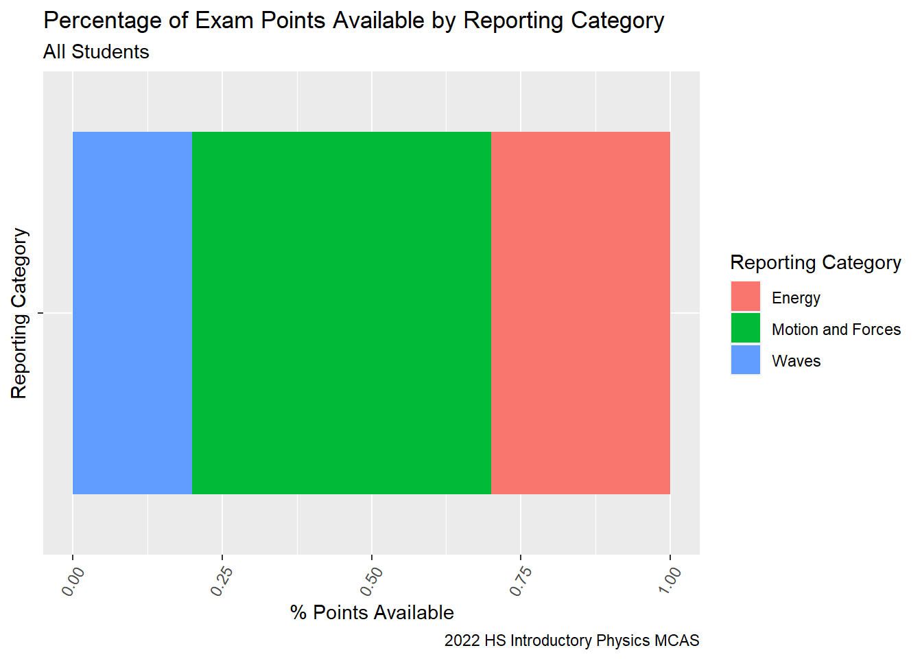
What reporting categories were emphasized by the state?
We can see from our summary that 50% of the exam points (30 of the available 60) come from questions from the Motion and Forces Reporting Category, followed by 30% from Energy, and 20% from Waves.
Code
SG9_Cat_Total<-SG9_Item%>%select(`sitem`, `item Possible Points`, `Reporting Category`)%>%group_by(`Reporting Category`)%>%summarise(available_points =sum(`item Possible Points`, na.rm=TRUE))%>%mutate(percent_available_points = available_points/(sum(available_points, na.rm =TRUE)))SG9_Cat_Total
Code
ggplot(SG9_Cat_Total, aes(x='',fill =`Reporting Category`, y =`available_points`)) +geom_bar(position="fill", stat ="identity") +coord_flip()+labs(subtitle ="All Students" ,y ="% Points Available",x="Reporting Category",title ="Percentage of Exam Points Available by Reporting Category",caption ="2022 HS Introductory Physics MCAS")+theme(axis.text.x=element_text(angle=60,hjust=1))
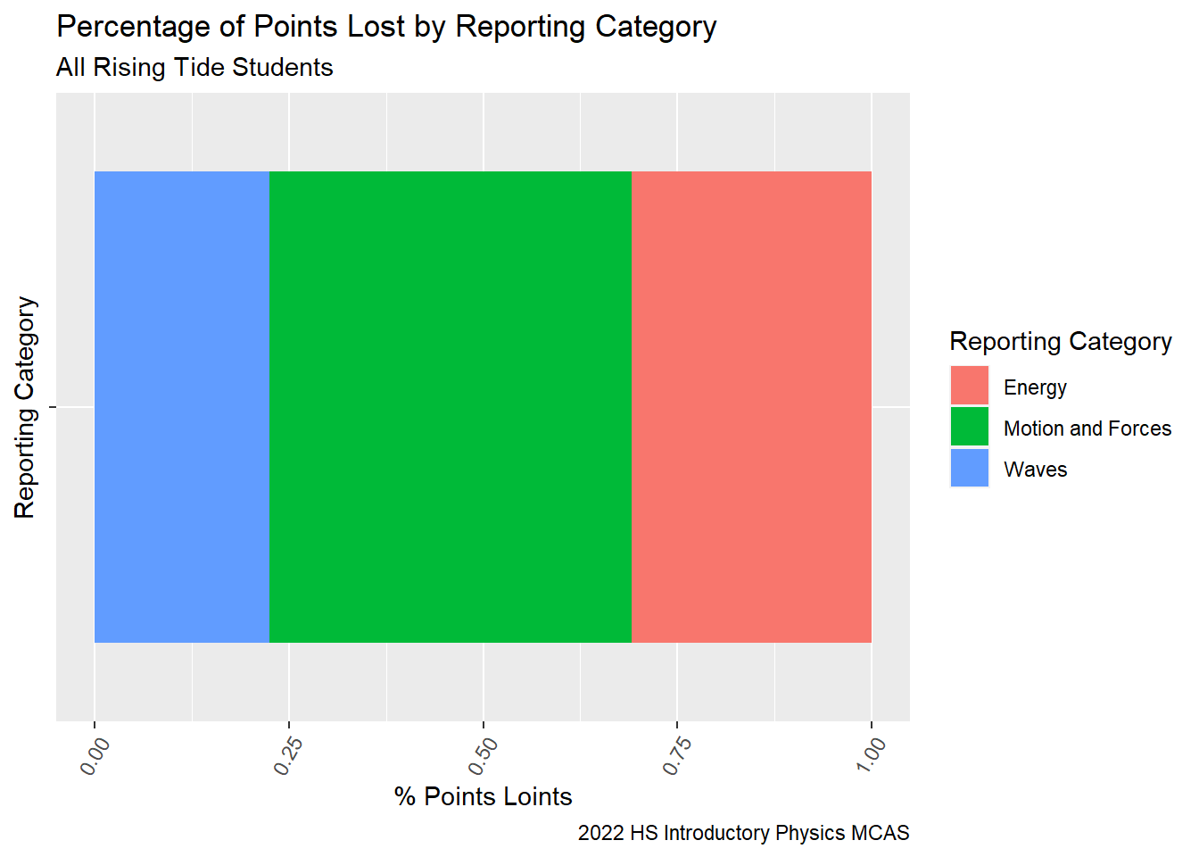
Where did Rising Tide students lose most of their points?
The proportion of points lost by Rising Tide students corresponds to the proportion of points available for each Reporting Category of the the exam. This suggests that our students are prepared consistently across the units in the Reporting Categories.
Code
SG9_Cat_Loss<-SG9_StudentItem%>%select(`sitem`, `Reporting Category`, `item Possible Points`, `sitem_score`)%>%group_by(`Reporting Category`)%>%summarise(sum_points_lost =sum(`item Possible Points`-`sitem_score`, na.rm=TRUE),available_points =sum(`item Possible Points`, na.rm=TRUE))%>%mutate(percent_points_lost =round(sum_points_lost/sum(sum_points_lost,na.rm=TRUE),2))%>%mutate(percent_available_points = available_points/(sum(available_points, na.rm =TRUE)))SG9_Cat_Loss<-SG9_Cat_Loss%>%select(`Reporting Category`, `percent_available_points`, `percent_points_lost`)SG9_Cat_Loss
Code
SG9_Percent_Loss<-SG9_StudentItem%>%select(`sitem`, `Reporting Category`, `item Possible Points`, `sitem_score`)%>%mutate(`points_lost`=`item Possible Points`-`sitem_score`)%>%#ggplot(df, aes(x='', fill=option)) + geom_bar(position = "fill") ggplot( aes(x='',fill =`Reporting Category`, y =`points_lost`)) +geom_bar(position="fill", stat ="identity") +coord_flip()+labs(subtitle ="All Rising Tide Students" ,y ="% Points Loints",x="Reporting Category",title ="Percentage of Points Lost by Reporting Category",caption ="2022 HS Introductory Physics MCAS")+theme(axis.text.x=element_text(angle=60,hjust=1))SG9_Percent_Loss
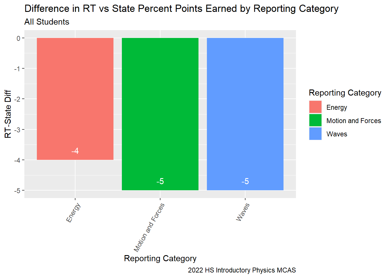
Did Rising Tide students’ performance relative to the state vary by content reporting categories?
We can see from our table that on average our students earned between 4 and 5 percent fewer of the available points relative to their peers in the state for items in each of the three reporting Categories.
Code
SG9_Cat_RTState<-SG9_Item%>%select(`sitem`, `item Possible Points`, `Reporting Category`, `State Percent Points`, `RT Percent Points`, `RT-State Diff`)%>%group_by(`Reporting Category`)%>%summarise(available_points =sum(`item Possible Points`, na.rm=TRUE),RT_points =sum(`RT Percent Points`*`item Possible Points`, na.rm =TRUE),RT_Percent_Points =100*round(RT_points/available_points,2),State_Percent_Points =100*round(sum(`State Percent Points`*`item Possible Points`/available_points, na.rm =TRUE),2))%>%mutate(`RT-State Diff`=round(RT_Percent_Points - State_Percent_Points, 2))%>%ggplot( aes(fill =`Reporting Category`, y=`RT-State Diff`, x=`Reporting Category`)) +geom_bar(position="dodge", stat="identity") +labs(subtitle ="All Students" ,y ="RT-State Diff",x="Reporting Category",title ="Difference in RT vs State Percent Points Earned by Reporting Category",caption ="2022 HS Introductory Physics MCAS")+theme(axis.text.x=element_text(angle=60,hjust=1))+geom_text(aes(label =`RT-State Diff`), vjust =-1., colour ="white", position =position_dodge(.9))SG9_Cat_RTState
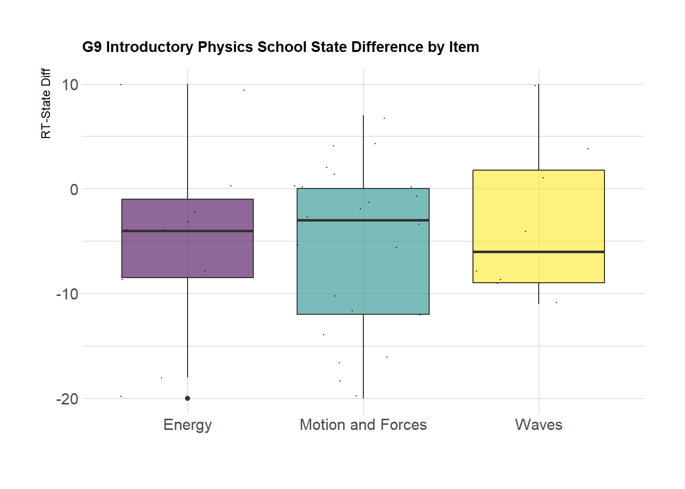
Here we see the distribution of RT-State Diff (difference between the percentage of points earned on a given item by Rising Tide students and percentage of points earned on the same item by their peers in the State) by sitem and content Reporting Category. We can see generally that items in the Motion and Forces Reporting Category seems to display the most concerning variability in student performance relative to the state. It would be worth looking at the specific question strands with the Physics Teachers. (It would be helpful to add item labels to the dots using ggplotly, however I did not find a way to have that render on the class blog)
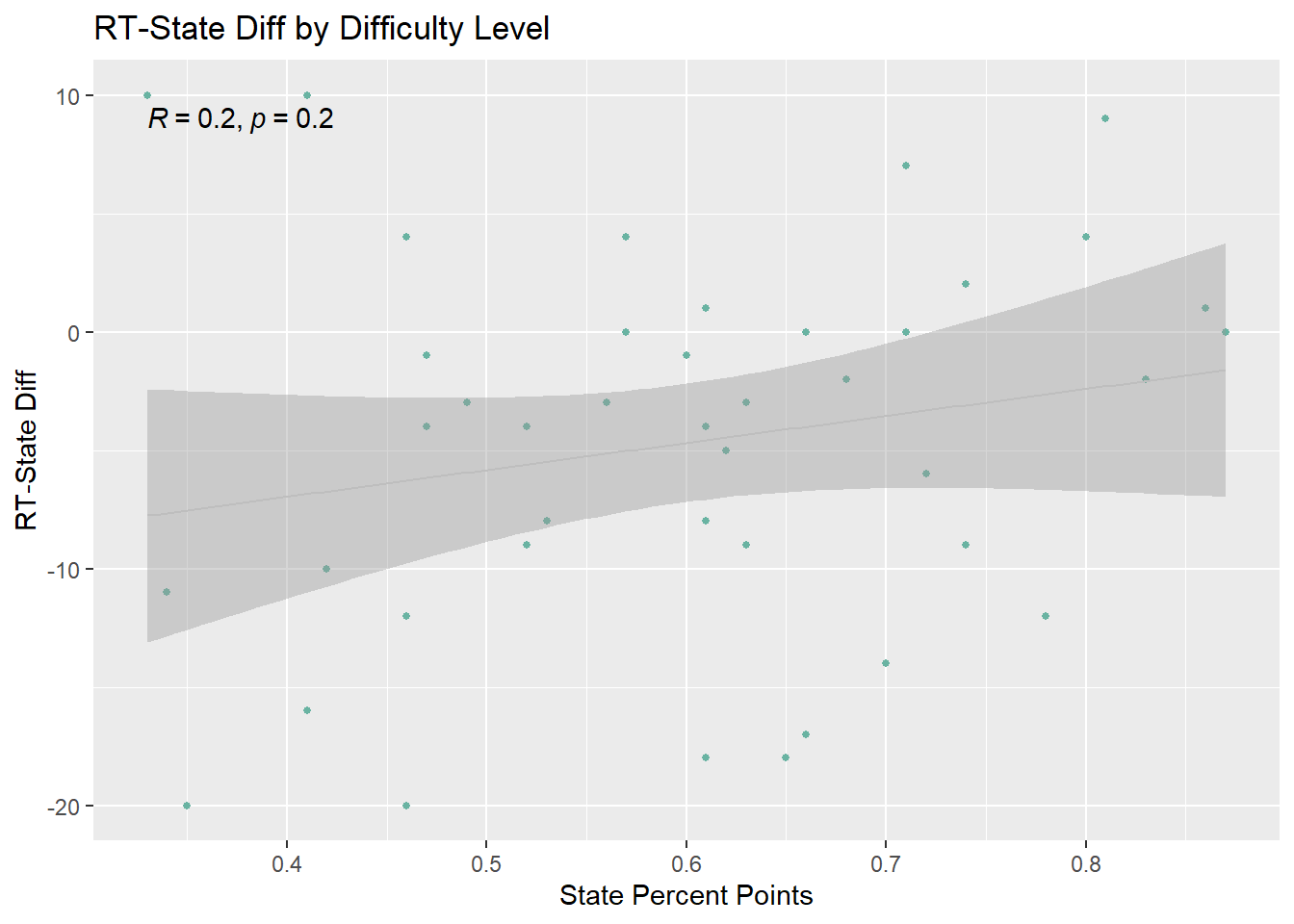
Can differences in Rising Tide student performance on an item and State performance on an item be explained by the difficulty level of an item?
When considering RT-State Diff against State Percent Points for each sitem on the MCAS, this does not seem to generally be the case. Although the regression line shows RT-State Diff more likely to be negative on items where students in the State earned fewer points, the p-value is not significant.
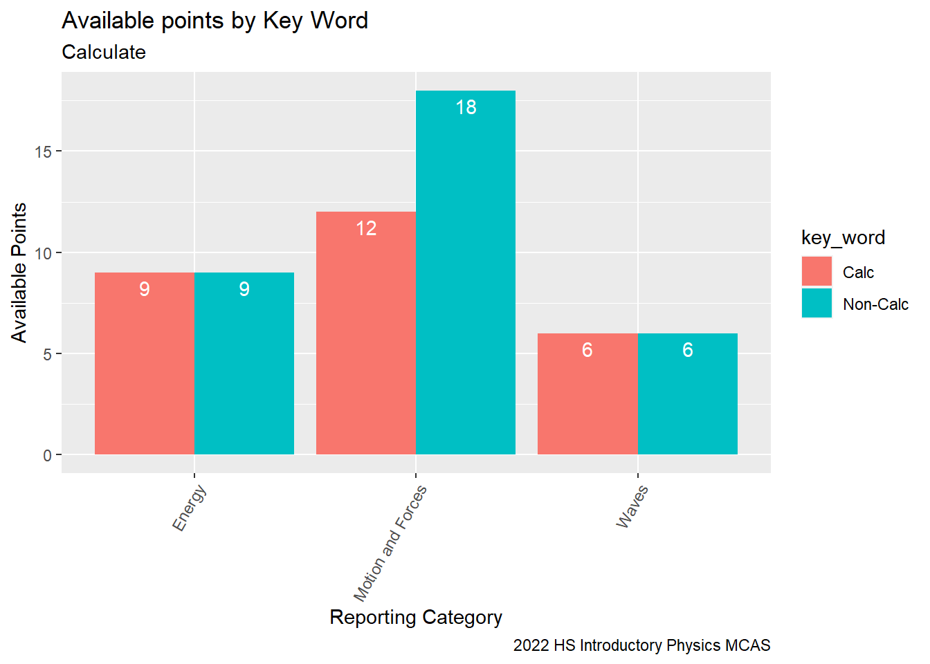
When scanning the item Desc entries in the SG9_Item data frame, there are several questions containing the word “Calculate” in their description.
How much is calculation emphasized on this exam and how did Rising Tide students perform relative to their peers in the state on items containing “calculate” in their description?
Now, we can see that by the Waves and Energy categories half of the available points come from questions with calculate and half do not. In the Motion and Forces category, 40% of points are associated with questions that ask students to “calculate”.
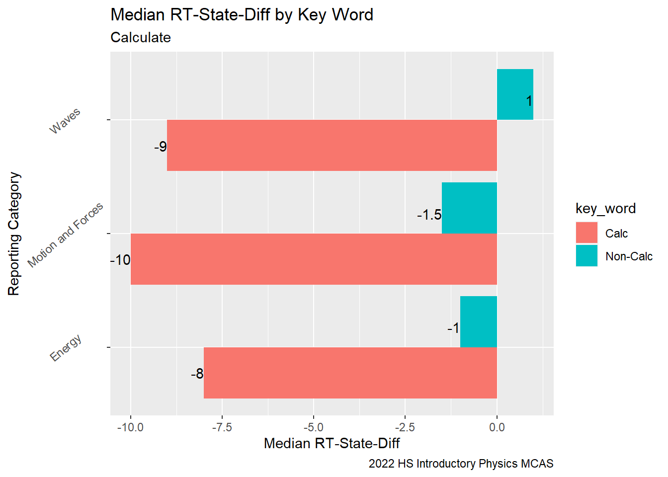
When we compare the median RT-State Diff for items containing the word “calculate” in their description vs. items that do not, we can see that across all of the Reporting Categories Rising Tide students performed significantly weaker relative to their peers in the state on questions that asked them to “calculate”.
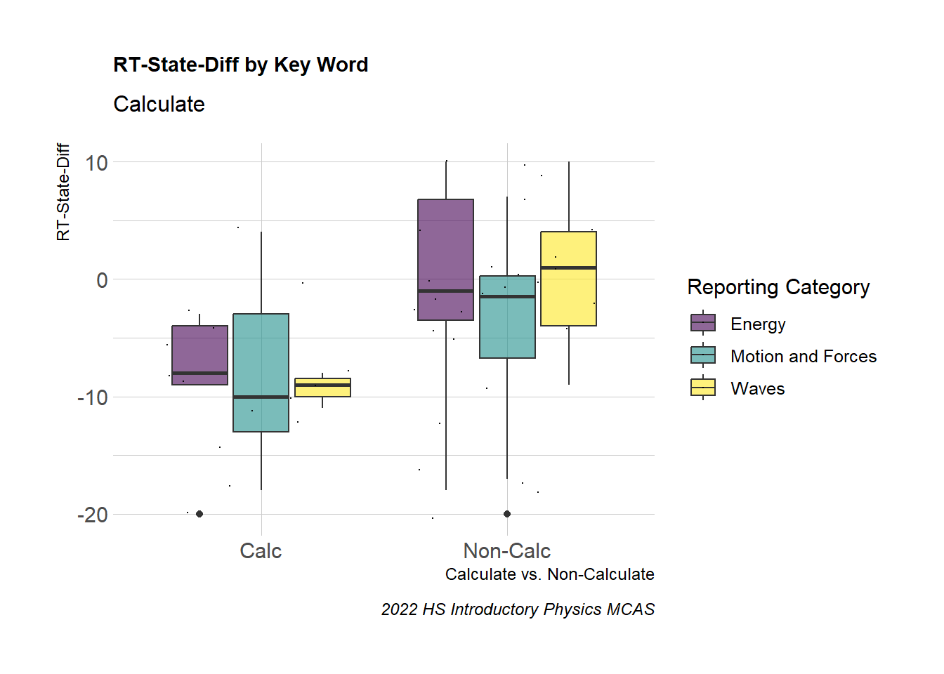
Here we can see the distribution of RT-State Diff by sitem and Reporting Category and the disparity in RT-State Diff when we consider items asking students to “Calculate” vs. those that do not.
Did RT students perform worse relative to their peers in the state on more “challenging” calculation items?
If we consider the difficulty of items containing the word calculate for students as reflected in the state-wide performance (State Percent Points) for a given item, the gap between Rising Tide students’ performance to their peers in the state RT-State Diff does not seem to increase significantly with the difficulty .
Code
#view(SG9_Calc)SG9_Calc_Dot<- SG9_Calc%>%select(`State Percent Points`, `RT-State Diff`, `key_word`)%>%filter(key_word =="Calc")%>%ggplot( aes(x=`State Percent Points`, y=`RT-State Diff`)) +geom_point(size =1, color="#69b3a2")+geom_smooth(method="lm",color="grey", size =.5 )+labs(title ="RT State Diff vs. State Percent Points", y ="RT State Diff",x ="State Percent Points")+stat_cor(method ="pearson")SG9_Calc_Dot
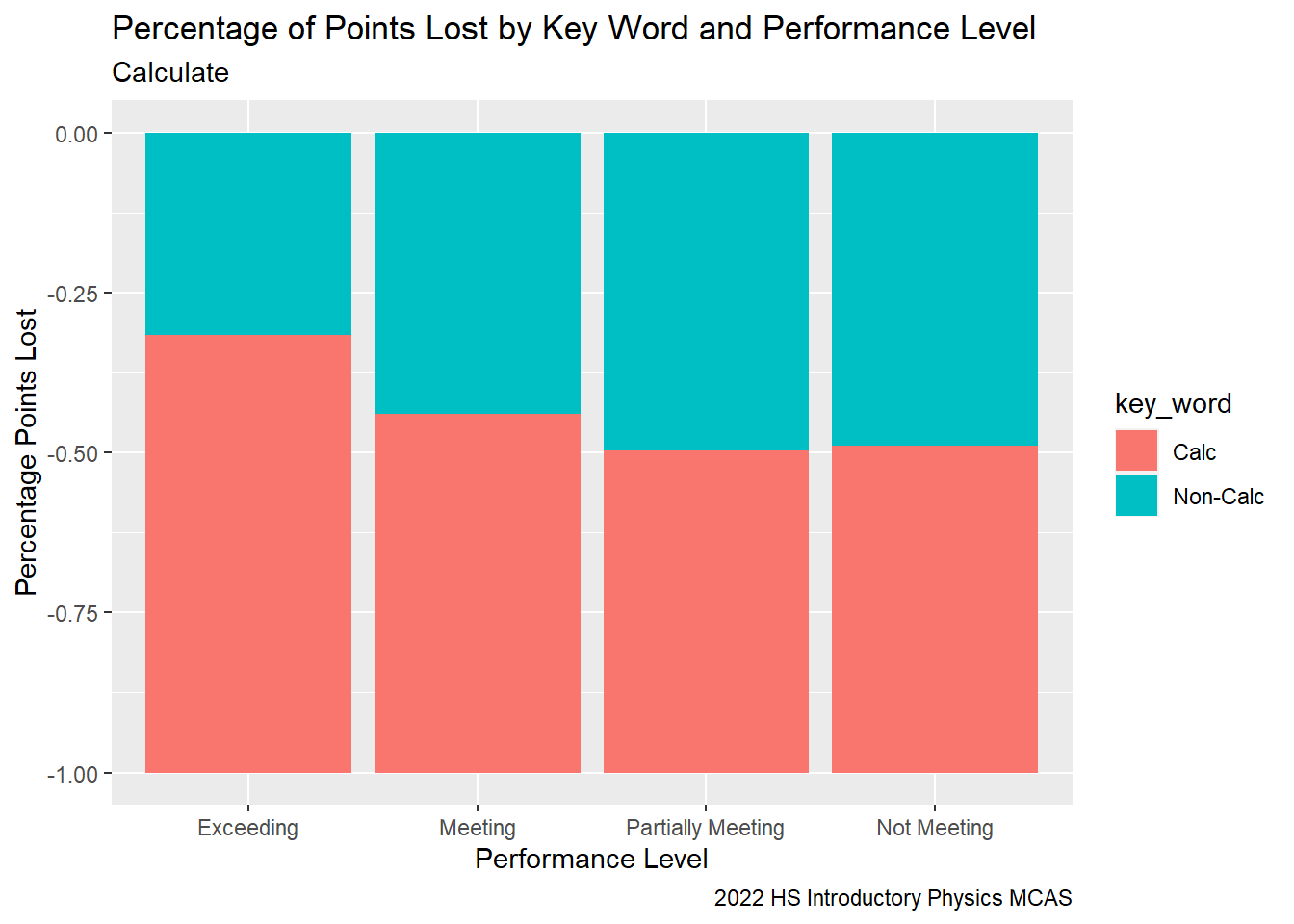
Is the “calculation gap” consistent across performance levels?
Here we can see that students with a higher performance level lost a greater proportion of their points on questions involving “Calculate”. I.e., the higher a student’s performance level, the greater the percentage of their points were lost to items asking them to “calculate”. This suggests that in the general classroom to raise student performance, students should spend a higher proportion of time on calculation based activities.
#view(SG9_StudentItem)G9Sci_StudentCalcPerflev%>%ggplot(aes(fill=`key_word`, y=total_points_lost, x=`sperflev`)) +geom_bar(position="fill", stat="identity") +labs(subtitle ="Calculate" ,y ="Percentage Points Lost",x="Performance Level",title ="Percentage of Points Lost by Key Word and Performance Level",caption ="2022 HS Introductory Physics MCAS")
Code
#G9Sci_StudentCalcPerflev
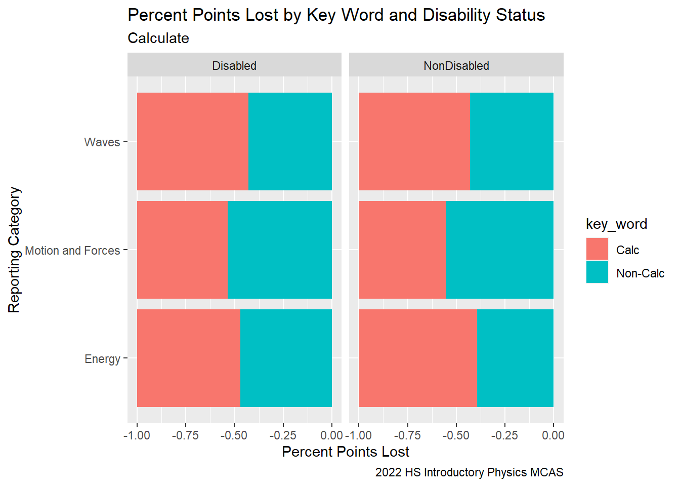
Are there differences in the performance of non-disabled and disabled students relative to their academic peers in the state?
We can see from our CU306 reports that our students with disabilities performed better relative to their peers in the state, RT-State Diff, across all Reporting Categories, while our non-disabled students performed worse relative to their peers in the state across all Reporting Categories. This suggest that more attention needs to be paid to the needs of the non-disabled students in the General Education setting.
When we examine the points lost by reporting category and disability status, there does not seem to be a significant difference in performance between disabled and non-disabled students across Reporting Categories.
Code
G9Sci_StudentCalcDis<-SG9_StudentItem%>%select(gender, sitem, sitem_score, `item Desc`, `item Possible Points`, `State Percent Points`, IEP, `RT-State Diff`, `Reporting Category`, `sperflev`)%>%mutate( key_word =case_when(!str_detect(`item Desc`, "calculate|Calculate") ~"Non-Calc",str_detect(`item Desc`, "calculate|Calculate") ~"Calc"))%>%group_by(`Reporting Category`, `key_word`, `IEP`)%>%summarise(total_points_lost =sum(`sitem_score`-`item Possible Points`, na.rm =TRUE))%>%ggplot(aes(fill=`key_word`, y=total_points_lost, x=`Reporting Category`)) +geom_bar(position="dodge", stat="identity")+facet_wrap(vars(IEP))+coord_flip()+labs(subtitle ="Calculate" ,y ="Sum Points Lost",x="Reporting Category",title ="Sum Points Lost by Key Word Non-Disabled vs. Disabled",caption ="2022 HS Introductory Physics MCAS")+geom_text(aes(label =`total_points_lost`), vjust =1.5, colour ="black", position =position_dodge(.95))#G9Sci_StudentCalcDis
Code
G9Sci_StudentCalcDis<-SG9_StudentItem%>%select(gender, sitem, sitem_score, `item Desc`, `item Possible Points`, `State Percent Points`, IEP, `RT-State Diff`, `Reporting Category`, `sperflev`)%>%mutate( key_word =case_when(!str_detect(`item Desc`, "calculate|Calculate") ~"Non-Calc",str_detect(`item Desc`, "calculate|Calculate") ~"Calc"))%>%group_by(`Reporting Category`, `key_word`, `IEP`)%>%summarise(sum_points_lost =sum(`sitem_score`-`item Possible Points`, na.rm =TRUE))%>%ggplot(aes(fill=`key_word`, y=sum_points_lost, x=`Reporting Category`)) +geom_bar(position="fill", stat="identity")+facet_wrap(vars(IEP))+coord_flip()+labs(subtitle ="Calculate" ,y ="Percent Points Lost",x="Reporting Category",title ="Percent Points Lost by Key Word and Disability Status",caption ="2022 HS Introductory Physics MCAS")G9Sci_StudentCalcDis
Conclusion
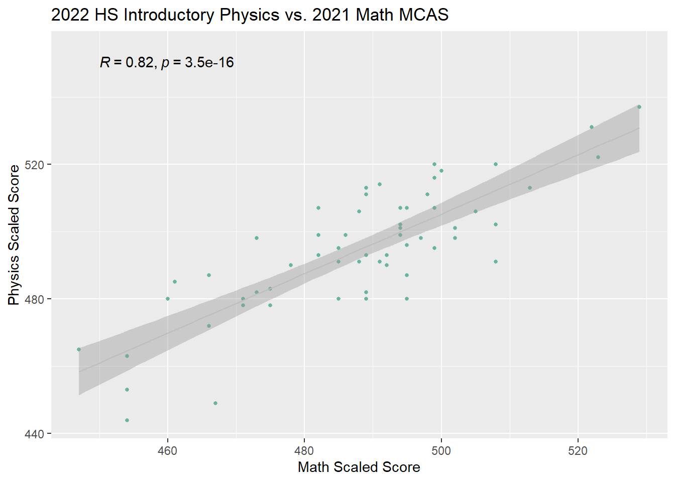
A student’s performance on their 9th Grade Introductory Physics MCAS is strongly associated with their performance on their 8th Grade Math MCAS exam. This suggests that the use of prior Math MCAS and current STAR Math testing data can identify students in need of extra support.
Code
SG9_Math<-MCAS_2022%>%select(sscaleds, mscaleds2021,sscaleds_prior, grade, sattempt)%>%filter((grade ==9) & sattempt !="N")%>%ggplot(aes(x=`mscaleds2021`, y =`sscaleds`))+geom_point(size =1, color="#69b3a2")+geom_smooth(method="lm",color="grey", size =.5 )+labs(title ="2022 HS Introductory Physics vs. 2021 Math MCAS", y ="Physics Scaled Score",x ="Math Scaled Score") +stat_cor(method ="pearson", label.x =450, label.y =550)SG9_Math
Rising Tide students as a whole performed slightly weaker relative to the state in all content reporting areas; however, students classified as disabled performed better relative to their peers in the state. The performance gap between Rising Tide students and students in the state on the HS Introductroy Physics exam is accounted for by the performance of the non-disabled students in the general classroom setting.
All Rising Tide students, regardless of disability status, performed significantly weaker relative to students in the State on items including the key word “Calculate” in their item description. This suggests that we should dedicate more classroom instructional time to problem solving with calculation. Notably, the higher a student’s performance level, the higher the percentage of points a student lost for calculation items. The largest area of growth for students across all performance categories is on calculation based items; evidence based math interventions include small group, differentiated problem sets.
The discrepancy in performance by Rising Tide students with and without disabilities relative to their associated academic peers in the state, suggest that our non-disabled students would benefit from some of the practices and supports currently provided to our students on IEPs. Differentiated, tiered, small group problem sets in the general classroom setting could potentially address the “calculation gap”.
Reflection: Limitations/Areas for Improvement
I was inspired to work on this report after years of experience working at a public school. Public education is a sector that is filled with passion and positive intentions but also divisive discussions. There exist a plethora of simplistic “one-trick fixes” that are marketed to students, teachers, and families. The use of data is the best tool we have against pressing forward and investing our precious time and money with initiatives that do not improve student outcomes.
Over the years, I’ve noticed that teachers and leaders are given annual data reports yet, most lack the time, capacity, or resources to identify evidence based, actionable measures to enact in the classroom or at the organizational level. When presented with all of the questions from an assessment individually and the performance of all of one’s students on paper, it is difficult to identify trends. Anecdotally, I have noticed every year the majority of teachers gravitating to the scores and performance of individual students that they previously taught and ascribing mistakes or successes to specific experiences with an individual or one word in a question prompt. While relationship building and teaching to a child are hallmarks to student-teacher relationships, a narrow lens like this will not allow a teacher to identify classroom level changes or curriculum level changes that could impact all students and future students. In one’s compassionate focus on individuals, a great opportunity to promote the learning for all students is lost.
With the use of R, and the MCAS reports, I decided to focus on ways to identify trends at the classroom or curricular level. I found it challenging to limit the scope of my work for this project. Also, I struggled with discerning when to use sum vs. when to use averages or medians. To improve a student’s performance on a test, we are concerned with total points lost and relative weight of a content category; to identify curricular weaknesses we are also interested in relative performance to the state by content area.
I only completed the analysis of the Introductory Physics Exam for High school students. I have ELA, Math, and Science results for grades 5-8 as well as grade 10. I am still working on building a general function library to generate similar graphics and tables for other content areas and grade levels and I would like to complete a similar report for each grade level and subject area assessment for teachers to use.
Given access to historical data, I think it would be beneficial to examine these trends over time to discern the performance gaps attributable to changes in the population of students (a factor which we cannot control or change) vs. those attributable to curriculum and teaching (an area we can influence and effect change).
I also have access to reports that include the teacher a student had and the grades they earned from their teacher in the year they were assessed on the MCAS. I would like to examine the relationship between a student’s performance as measured by their teachers compared to their performance level as measured by the state. Are their patterns to the groups of students with the largest discrepancy between these two metrics? This would be important data to support the teaching and learning at our school.
On a broader scale, I think that I need to develop a stronger sense for what summary statistics are the most meaningful for a given variable to identify potential trends or insights and subsequently what visualizations best convey these insights to a reader. I would also like to develop a tool-kit of best practices for “checking against my own biases”. What set of metrics can I perform to best control for my potential mistakes as a human being with a limited perspective?
Note
I did not cite the source for the MCAS Preliminary Results because it is not a publicly available data set as it contains students’ personal information. I did use the raw csv. file retrievable from the DESE portal title “MCAS Full Preliminary Results”.
References
Chang, W. (2022). R Graphics Cookbook, 2nd Edition. O’Reilly Media.
Grolemund, G., & Wickham, H. (2016). R for Data Science: Import, Tidy, Transform, Visualize, and Model Data. O’Reilly Media.
H. Wickham. ggplot2: Elegant Graphics for Data Analysis. Springer-Verlag New York, 2009.
Papay, J. P., Mantil, A., McDonough, A., Donahue, K., An, L., & Murnane, R. J. (n.d.). Lifting all boats? Accomplishments and Challenges from 20 Years of Education Reform in Massachusetts. Retrieved December 2, 2022, from https://annenberg.brown.edu/sites/default/files/LiftingAllBoats_FINAL.pdf
R Core Team. (2020). R: A language and environment for statistical computing. R Foundation for Statistical Computing, Vienna, Austria.https://www.r-project.org.
RStudio Team. (2019). RStudio: Integrated Development for R. RStudio, Inc., Boston, MA. https://www.rstudio.com.
Wickham H, Averick M, Bryan J, Chang W, McGowan LD, François R, Grolemund G, Hayes A, Henry L, Hester J, Kuhn M, Pedersen TL, Miller E, Bache SM, Müller K, Ooms J, Robinson D, Seidel DP, Spinu V, Takahashi K, Vaughan D, Wilke C, Woo K, Yutani H (2019). “Welcome to the tidyverse.” Journal of Open Source Software, 4(43), 1686. doi:10.21105/joss.01686 https://doi.org/10.21105/joss.01686.
Percent of points earned by Massachusetts students for a given sitem
Code
# examine the summary to decide how to best set up our data frameprint(summarytools::dfSummary(MCAS_2022,varnumbers =FALSE,plain.ascii =FALSE,style ="grid",graph.magnif =0.70,valid.col =FALSE),method ='render',table.classes ='table-condensed')
Data Frame Summary
MCAS_2022
Dimensions: 495 x 256
Duplicates: 0
Variable
Stats / Values
Freqs (% of Valid)
Graph
Missing
adminyear
[numeric]
1 distinct value
2022
:
495
(
100.0%
)
0
(0.0%)
testschoolcode
[character]
1. 4830305
495
(
100.0%
)
0
(0.0%)
grade
[factor]
1. 5
2. 6
3. 7
4. 8
5. 9
6. 10
89
(
18.0%
)
91
(
18.4%
)
92
(
18.6%
)
91
(
18.4%
)
69
(
13.9%
)
63
(
12.7%
)
0
(0.0%)
gradesims
[numeric]
Mean (sd) : 7.3 (1.6)
min ≤ med ≤ max:
5 ≤ 7 ≤ 10
IQR (CV) : 3 (0.2)
5
:
89
(
18.0%
)
6
:
91
(
18.4%
)
7
:
92
(
18.6%
)
8
:
91
(
18.4%
)
9
:
69
(
13.9%
)
10
:
63
(
12.7%
)
0
(0.0%)
dob
[Date]
min : 2005-02-08
med : 2008-11-29
max : 2011-10-17
range : 6y 8m 9d
427 distinct values
0
(0.0%)
gender
[character]
1. F
2. M
3. N
242
(
48.9%
)
251
(
50.7%
)
2
(
0.4%
)
0
(0.0%)
race
[character]
1. A
2. B
3. H
4. M
5. N
6. W
8
(
1.6%
)
6
(
1.2%
)
25
(
5.1%
)
41
(
8.3%
)
5
(
1.0%
)
410
(
82.8%
)
0
(0.0%)
yrsinmass
[character]
1. 1
2. 2
3. 3
4. 4
5. 5+
11
(
2.2%
)
18
(
3.6%
)
19
(
3.8%
)
16
(
3.2%
)
431
(
87.1%
)
0
(0.0%)
yrsinmass_num
[numeric]
Mean (sd) : 7.3 (2.4)
min ≤ med ≤ max:
1 ≤ 8 ≤ 12
IQR (CV) : 3 (0.3)
12 distinct values
0
(0.0%)
yrsinsch
[numeric]
Mean (sd) : 2.6 (1.5)
min ≤ med ≤ max:
1 ≤ 2 ≤ 6
IQR (CV) : 3 (0.6)
1
:
159
(
32.1%
)
2
:
116
(
23.4%
)
3
:
80
(
16.2%
)
4
:
77
(
15.6%
)
5
:
31
(
6.3%
)
6
:
32
(
6.5%
)
0
(0.0%)
highneeds
[character]
1. 0
2. 1
290
(
58.6%
)
205
(
41.4%
)
0
(0.0%)
lowincome
[character]
1. 0
2. 1
369
(
74.5%
)
126
(
25.5%
)
0
(0.0%)
title1
[character]
1. 0
2. 1
393
(
79.4%
)
102
(
20.6%
)
0
(0.0%)
ever_EL
[character]
1. 1
20
(
100.0%
)
475
(96.0%)
EL
[character]
1. 0
2. 1
488
(
98.6%
)
7
(
1.4%
)
0
(0.0%)
EL_FormerEL
[character]
1. 0
2. 1
480
(
97.0%
)
15
(
3.0%
)
0
(0.0%)
FormerEL
[character]
1. 0
2. 1
487
(
98.4%
)
8
(
1.6%
)
0
(0.0%)
ELfirstyear
[character]
All NA's
495
(100.0%)
IEP
[character]
1. Disabled
2. NonDisabled
114
(
23.0%
)
381
(
77.0%
)
0
(0.0%)
plan504
[character]
1. 0
2. 1
443
(
89.5%
)
52
(
10.5%
)
0
(0.0%)
firstlanguage
[character]
1. 2
2. 267
3. 415
4. 6
5. 630
6. 7
7. 759
1
(
0.2%
)
481
(
97.2%
)
2
(
0.4%
)
8
(
1.6%
)
1
(
0.2%
)
1
(
0.2%
)
1
(
0.2%
)
0
(0.0%)
natureofdis
[numeric]
Mean (sd) : 6.9 (1.9)
min ≤ med ≤ max:
2 ≤ 7 ≤ 12
IQR (CV) : 3 (0.3)
2
:
1
(
0.9%
)
3
:
9
(
7.8%
)
4
:
1
(
0.9%
)
5
:
19
(
16.5%
)
7
:
40
(
34.8%
)
8
:
38
(
33.0%
)
11
:
5
(
4.3%
)
12
:
2
(
1.7%
)
380
(76.8%)
levelofneed
[factor]
1. 1
2. 2
3. 3
4. 4
3
(
2.6%
)
14
(
12.2%
)
97
(
84.3%
)
1
(
0.9%
)
380
(76.8%)
spedplacement
[character]
1. 0
2. 1
3. 10
4. 20
380
(
76.8%
)
1
(
0.2%
)
104
(
21.0%
)
10
(
2.0%
)
0
(0.0%)
town
[character]
1. 239
2. 310
3. 52
4. 145
5. 182
6. 36
7. 20
8. 261
9. 171
10. 231
[ 11 others ]
257
(
51.9%
)
54
(
10.9%
)
33
(
6.7%
)
30
(
6.1%
)
23
(
4.6%
)
20
(
4.0%
)
18
(
3.6%
)
12
(
2.4%
)
11
(
2.2%
)
8
(
1.6%
)
29
(
5.9%
)
0
(0.0%)
county
[character]
1. Barnstable
2. Plymouth
56
(
11.3%
)
439
(
88.7%
)
0
(0.0%)
octenr
[numeric]
Min : 0
Mean : 1
Max : 1
0
:
13
(
2.6%
)
1
:
482
(
97.4%
)
0
(0.0%)
conenr_sch
[numeric]
1 distinct value
1
:
55
(
100.0%
)
440
(88.9%)
conenr_sta
[numeric]
1 distinct value
1
:
61
(
100.0%
)
434
(87.7%)
access_part
[numeric]
1 distinct value
1
:
7
(
100.0%
)
488
(98.6%)
ealt
[logical]
All NA's
495
(100.0%)
ecomplexity
[logical]
All NA's
495
(100.0%)
emode
[character]
1. O
422
(
100.0%
)
73
(14.7%)
eteststat
[character]
1. NTA
2. NTO
3. T
4
(
0.9%
)
1
(
0.2%
)
421
(
98.8%
)
69
(13.9%)
wptopdev
[logical]
All NA's
495
(100.0%)
wpcompconv
[logical]
All NA's
495
(100.0%)
eitem1
[numeric]
Min : 0
Mean : 0.8
Max : 1
0
:
95
(
22.6%
)
1
:
326
(
77.4%
)
74
(14.9%)
eitem2
[numeric]
Min : 0
Mean : 0.7
Max : 1
0
:
132
(
31.4%
)
1
:
289
(
68.6%
)
74
(14.9%)
eitem3
[numeric]
Min : 0
Mean : 0.8
Max : 1
0
:
91
(
21.6%
)
1
:
330
(
78.4%
)
74
(14.9%)
eitem4
[numeric]
Min : 0
Mean : 0.8
Max : 1
0
:
79
(
18.8%
)
1
:
342
(
81.2%
)
74
(14.9%)
eitem5
[numeric]
Mean (sd) : 0.9 (0.6)
min ≤ med ≤ max:
0 ≤ 1 ≤ 2
IQR (CV) : 1 (0.7)
0
:
109
(
25.9%
)
1
:
246
(
58.4%
)
2
:
66
(
15.7%
)
74
(14.9%)
eitem6
[numeric]
Min : 0
Mean : 0.8
Max : 1
0
:
97
(
23.0%
)
1
:
324
(
77.0%
)
74
(14.9%)
eitem7
[numeric]
Mean (sd) : 0.8 (0.5)
min ≤ med ≤ max:
0 ≤ 1 ≤ 2
IQR (CV) : 0 (0.6)
0
:
95
(
22.6%
)
1
:
307
(
72.9%
)
2
:
19
(
4.5%
)
74
(14.9%)
eitem8
[numeric]
Mean (sd) : 0.8 (0.5)
min ≤ med ≤ max:
0 ≤ 1 ≤ 2
IQR (CV) : 0 (0.6)
0
:
102
(
24.2%
)
1
:
292
(
69.4%
)
2
:
27
(
6.4%
)
74
(14.9%)
eitem9
[numeric]
Mean (sd) : 1.3 (1.5)
min ≤ med ≤ max:
0 ≤ 1 ≤ 7
IQR (CV) : 0 (1.2)
0
:
79
(
18.8%
)
1
:
285
(
67.7%
)
2
:
10
(
2.4%
)
4
:
20
(
4.8%
)
6
:
20
(
4.8%
)
7
:
7
(
1.7%
)
74
(14.9%)
eitem10
[numeric]
Mean (sd) : 1.2 (0.8)
min ≤ med ≤ max:
0 ≤ 1 ≤ 2
IQR (CV) : 2 (0.7)
0
:
107
(
25.4%
)
1
:
124
(
29.5%
)
2
:
190
(
45.1%
)
74
(14.9%)
eitem11
[numeric]
Mean (sd) : 1.2 (0.7)
min ≤ med ≤ max:
0 ≤ 1 ≤ 2
IQR (CV) : 1 (0.5)
0
:
54
(
12.8%
)
1
:
208
(
49.4%
)
2
:
159
(
37.8%
)
74
(14.9%)
eitem12
[numeric]
Mean (sd) : 2.5 (2.3)
min ≤ med ≤ max:
0 ≤ 1 ≤ 8
IQR (CV) : 3 (0.9)
0
:
69
(
16.4%
)
1
:
152
(
36.1%
)
2
:
33
(
7.8%
)
3
:
6
(
1.4%
)
4
:
80
(
19.0%
)
5
:
7
(
1.7%
)
6
:
50
(
11.9%
)
7
:
18
(
4.3%
)
8
:
6
(
1.4%
)
74
(14.9%)
eitem13
[numeric]
Mean (sd) : 1.4 (1.5)
min ≤ med ≤ max:
0 ≤ 1 ≤ 7
IQR (CV) : 1 (1)
0
:
88
(
21.0%
)
1
:
218
(
51.9%
)
2
:
56
(
13.3%
)
3
:
8
(
1.9%
)
4
:
27
(
6.4%
)
5
:
3
(
0.7%
)
6
:
18
(
4.3%
)
7
:
2
(
0.5%
)
75
(15.2%)
eitem14
[numeric]
Min : 0
Mean : 0.8
Max : 1
0
:
104
(
24.6%
)
1
:
318
(
75.4%
)
73
(14.7%)
eitem15
[numeric]
Mean (sd) : 0.9 (0.6)
min ≤ med ≤ max:
0 ≤ 1 ≤ 2
IQR (CV) : 0 (0.7)
0
:
101
(
23.9%
)
1
:
260
(
61.6%
)
2
:
61
(
14.5%
)
73
(14.7%)
eitem16
[numeric]
Min : 0
Mean : 0.8
Max : 1
0
:
76
(
18.0%
)
1
:
346
(
82.0%
)
73
(14.7%)
eitem17
[numeric]
Min : 0
Mean : 0.7
Max : 1
0
:
122
(
28.9%
)
1
:
300
(
71.1%
)
73
(14.7%)
eitem18
[numeric]
Min : 0
Mean : 0.7
Max : 1
0
:
110
(
26.1%
)
1
:
312
(
73.9%
)
73
(14.7%)
eitem19
[numeric]
Mean (sd) : 0.9 (0.7)
min ≤ med ≤ max:
0 ≤ 1 ≤ 2
IQR (CV) : 1 (0.7)
0
:
110
(
26.1%
)
1
:
234
(
55.5%
)
2
:
78
(
18.5%
)
73
(14.7%)
eitem20
[numeric]
Mean (sd) : 1 (0.6)
min ≤ med ≤ max:
0 ≤ 1 ≤ 2
IQR (CV) : 0 (0.6)
0
:
61
(
14.5%
)
1
:
281
(
66.6%
)
2
:
80
(
19.0%
)
73
(14.7%)
eitem21
[numeric]
Mean (sd) : 1 (0.5)
min ≤ med ≤ max:
0 ≤ 1 ≤ 2
IQR (CV) : 0 (0.5)
0
:
64
(
15.2%
)
1
:
309
(
73.2%
)
2
:
49
(
11.6%
)
73
(14.7%)
eitem22
[numeric]
Mean (sd) : 1.4 (1.5)
min ≤ med ≤ max:
0 ≤ 1 ≤ 7
IQR (CV) : 0 (1.1)
0
:
51
(
12.1%
)
1
:
310
(
73.5%
)
2
:
10
(
2.4%
)
4
:
23
(
5.5%
)
6
:
19
(
4.5%
)
7
:
9
(
2.1%
)
73
(14.7%)
eitem23
[numeric]
Mean (sd) : 0.8 (0.6)
min ≤ med ≤ max:
0 ≤ 1 ≤ 2
IQR (CV) : 1 (0.7)
0
:
124
(
29.4%
)
1
:
252
(
59.7%
)
2
:
46
(
10.9%
)
73
(14.7%)
eitem24
[numeric]
Mean (sd) : 0.9 (0.6)
min ≤ med ≤ max:
0 ≤ 1 ≤ 2
IQR (CV) : 0 (0.6)
0
:
81
(
19.2%
)
1
:
287
(
68.0%
)
2
:
54
(
12.8%
)
73
(14.7%)
eitem25
[numeric]
Mean (sd) : 0.9 (0.6)
min ≤ med ≤ max:
0 ≤ 1 ≤ 2
IQR (CV) : 0 (0.6)
0
:
84
(
19.9%
)
1
:
285
(
67.5%
)
2
:
53
(
12.6%
)
73
(14.7%)
eitem26
[numeric]
Min : 0
Mean : 0.7
Max : 1
0
:
121
(
28.7%
)
1
:
301
(
71.3%
)
73
(14.7%)
eitem27
[numeric]
Mean (sd) : 0.9 (0.6)
min ≤ med ≤ max:
0 ≤ 1 ≤ 2
IQR (CV) : 0 (0.6)
0
:
89
(
21.1%
)
1
:
272
(
64.5%
)
2
:
61
(
14.5%
)
73
(14.7%)
eitem28
[numeric]
Mean (sd) : 0.9 (0.6)
min ≤ med ≤ max:
0 ≤ 1 ≤ 2
IQR (CV) : 0 (0.6)
0
:
86
(
20.4%
)
1
:
283
(
67.1%
)
2
:
53
(
12.6%
)
73
(14.7%)
eitem29
[numeric]
Mean (sd) : 0.8 (0.6)
min ≤ med ≤ max:
0 ≤ 1 ≤ 2
IQR (CV) : 1 (0.7)
0
:
123
(
29.1%
)
1
:
256
(
60.7%
)
2
:
43
(
10.2%
)
73
(14.7%)
eitem30
[numeric]
Mean (sd) : 1.2 (0.7)
min ≤ med ≤ max:
0 ≤ 1 ≤ 2
IQR (CV) : 1 (0.6)
0
:
67
(
15.9%
)
1
:
219
(
51.9%
)
2
:
136
(
32.2%
)
73
(14.7%)
eitem31
[numeric]
Mean (sd) : 3.2 (2.2)
min ≤ med ≤ max:
0 ≤ 3 ≤ 8
IQR (CV) : 4 (0.7)
0
:
25
(
6.9%
)
1
:
70
(
19.4%
)
2
:
81
(
22.5%
)
3
:
21
(
5.8%
)
4
:
69
(
19.2%
)
5
:
14
(
3.9%
)
6
:
55
(
15.3%
)
7
:
17
(
4.7%
)
8
:
8
(
2.2%
)
135
(27.3%)
eitem32
[numeric]
Mean (sd) : 3.2 (1.7)
min ≤ med ≤ max:
0 ≤ 3.5 ≤ 8
IQR (CV) : 2 (0.5)
0
:
5
(
5.4%
)
1
:
5
(
5.4%
)
2
:
32
(
34.8%
)
3
:
4
(
4.3%
)
4
:
34
(
37.0%
)
5
:
1
(
1.1%
)
6
:
10
(
10.9%
)
8
:
1
(
1.1%
)
403
(81.4%)
eitem33
[logical]
All NA's
495
(100.0%)
eitem34
[logical]
All NA's
495
(100.0%)
eitem35
[logical]
All NA's
495
(100.0%)
eitem36
[logical]
All NA's
495
(100.0%)
eitem37
[logical]
All NA's
495
(100.0%)
eitem38
[logical]
All NA's
495
(100.0%)
eitem39
[logical]
All NA's
495
(100.0%)
eitem40
[logical]
All NA's
495
(100.0%)
erawsc
[numeric]
Mean (sd) : 33 (8.2)
min ≤ med ≤ max:
6 ≤ 34 ≤ 47
IQR (CV) : 10 (0.2)
39 distinct values
73
(14.7%)
emcpts
[numeric]
Mean (sd) : 18.3 (4.1)
min ≤ med ≤ max:
3 ≤ 19 ≤ 26
IQR (CV) : 5 (0.2)
24 distinct values
73
(14.7%)
eorpts
[numeric]
Mean (sd) : 14.7 (5.4)
min ≤ med ≤ max:
1 ≤ 15 ≤ 28
IQR (CV) : 8 (0.4)
28 distinct values
73
(14.7%)
eperpospts
[numeric]
Mean (sd) : 66.3 (16.3)
min ≤ med ≤ max:
12 ≤ 69 ≤ 94
IQR (CV) : 20 (0.2)
63 distinct values
73
(14.7%)
escaleds
[numeric]
Mean (sd) : 501.3 (18.5)
min ≤ med ≤ max:
442 ≤ 502 ≤ 545
IQR (CV) : 25 (0)
74 distinct values
74
(14.9%)
eperflev
[ordered, factor]
1. E
2. M
3. PM
4. NM
5. DNT
6. ABS
24
(
5.6%
)
206
(
48.4%
)
169
(
39.7%
)
22
(
5.2%
)
1
(
0.2%
)
4
(
0.9%
)
69
(13.9%)
eperf2
[ordered, factor]
1. Exceeding
2. Meeting
3. Partially Meeting
4. Not Meeting
24
(
5.7%
)
206
(
48.9%
)
169
(
40.1%
)
22
(
5.2%
)
74
(14.9%)
enumin
[numeric]
1 distinct value
1
:
421
(
100.0%
)
74
(14.9%)
eassess
[numeric]
Min : 0
Mean : 1
Max : 1
0
:
4
(
0.9%
)
1
:
421
(
99.1%
)
70
(14.1%)
esgp
[numeric]
Mean (sd) : 52.6 (29.6)
min ≤ med ≤ max:
1 ≤ 54 ≤ 99
IQR (CV) : 48.5 (0.6)
96 distinct values
109
(22.0%)
idea1
[character]
1. 0
2. 1
3. 2
4. 3
5. 4
6. 5
7. BL
8. OT
70
(
16.4%
)
79
(
18.5%
)
138
(
32.4%
)
97
(
22.8%
)
27
(
6.3%
)
6
(
1.4%
)
7
(
1.6%
)
2
(
0.5%
)
69
(13.9%)
conv1
[character]
1. 0
2. 1
3. 2
4. 3
5. BL
6. OT
34
(
8.0%
)
121
(
28.4%
)
140
(
32.9%
)
122
(
28.6%
)
7
(
1.6%
)
2
(
0.5%
)
69
(13.9%)
idea2
[character]
1. 0
2. 1
3. 2
4. 3
5. 4
6. 5
7. BL
8. OT
21
(
4.9%
)
121
(
28.4%
)
146
(
34.3%
)
96
(
22.5%
)
27
(
6.3%
)
9
(
2.1%
)
4
(
0.9%
)
2
(
0.5%
)
69
(13.9%)
conv2
[character]
1. 0
2. 1
3. 2
4. 3
5. BL
6. OT
33
(
7.7%
)
121
(
28.4%
)
145
(
34.0%
)
121
(
28.4%
)
4
(
0.9%
)
2
(
0.5%
)
69
(13.9%)
idea3
[logical]
All NA's
495
(100.0%)
conv3
[logical]
All NA's
495
(100.0%)
eattempt
[character]
1. F
2. N
3. P
421
(
98.8%
)
4
(
0.9%
)
1
(
0.2%
)
69
(13.9%)
malt
[logical]
All NA's
495
(100.0%)
mcomplexity
[logical]
All NA's
495
(100.0%)
mmode
[character]
1. O
424
(
100.0%
)
71
(14.3%)
mteststat
[character]
1. NTA
2. NTO
3. T
2
(
0.5%
)
1
(
0.2%
)
423
(
99.3%
)
69
(13.9%)
mitem1
[numeric]
Min : 0
Mean : 0.8
Max : 1
0
:
94
(
22.3%
)
1
:
328
(
77.7%
)
73
(14.7%)
mitem2
[numeric]
Min : 0
Mean : 0.7
Max : 1
0
:
127
(
30.1%
)
1
:
295
(
69.9%
)
73
(14.7%)
mitem3
[numeric]
Min : 0
Mean : 0.6
Max : 1
0
:
174
(
41.2%
)
1
:
248
(
58.8%
)
73
(14.7%)
mitem4
[numeric]
Mean (sd) : 1.1 (1.1)
min ≤ med ≤ max:
0 ≤ 1 ≤ 4
IQR (CV) : 2 (1)
0
:
156
(
37.1%
)
1
:
148
(
35.2%
)
2
:
55
(
13.1%
)
3
:
42
(
10.0%
)
4
:
19
(
4.5%
)
75
(15.2%)
mitem5
[numeric]
Min : 0
Mean : 0.4
Max : 1
0
:
237
(
56.3%
)
1
:
184
(
43.7%
)
74
(14.9%)
mitem6
[numeric]
Mean (sd) : 0.9 (0.9)
min ≤ med ≤ max:
0 ≤ 1 ≤ 4
IQR (CV) : 1 (1)
0
:
151
(
35.8%
)
1
:
219
(
51.9%
)
2
:
19
(
4.5%
)
3
:
22
(
5.2%
)
4
:
11
(
2.6%
)
73
(14.7%)
mitem7
[numeric]
Mean (sd) : 0.6 (0.7)
min ≤ med ≤ max:
0 ≤ 0 ≤ 2
IQR (CV) : 1 (1.1)
0
:
213
(
50.5%
)
1
:
159
(
37.7%
)
2
:
50
(
11.8%
)
73
(14.7%)
mitem8
[numeric]
Mean (sd) : 0.8 (0.9)
min ≤ med ≤ max:
0 ≤ 1 ≤ 4
IQR (CV) : 1 (1.1)
0
:
182
(
43.4%
)
1
:
167
(
39.9%
)
2
:
54
(
12.9%
)
3
:
7
(
1.7%
)
4
:
9
(
2.1%
)
76
(15.4%)
mitem9
[numeric]
Mean (sd) : 0.8 (0.9)
min ≤ med ≤ max:
0 ≤ 1 ≤ 4
IQR (CV) : 1 (1)
0
:
150
(
35.5%
)
1
:
225
(
53.3%
)
2
:
27
(
6.4%
)
3
:
8
(
1.9%
)
4
:
12
(
2.8%
)
73
(14.7%)
mitem10
[numeric]
Min : 0
Mean : 0.6
Max : 1
0
:
183
(
43.4%
)
1
:
239
(
56.6%
)
73
(14.7%)
mitem11
[numeric]
Mean (sd) : 0.7 (0.5)
min ≤ med ≤ max:
0 ≤ 1 ≤ 2
IQR (CV) : 1 (0.7)
0
:
123
(
29.1%
)
1
:
288
(
68.2%
)
2
:
11
(
2.6%
)
73
(14.7%)
mitem12
[numeric]
Mean (sd) : 0.8 (0.8)
min ≤ med ≤ max:
0 ≤ 1 ≤ 4
IQR (CV) : 1 (1)
0
:
161
(
38.2%
)
1
:
222
(
52.6%
)
2
:
23
(
5.5%
)
3
:
9
(
2.1%
)
4
:
7
(
1.7%
)
73
(14.7%)
mitem13
[numeric]
Mean (sd) : 1.2 (1.3)
min ≤ med ≤ max:
0 ≤ 1 ≤ 4
IQR (CV) : 1 (1.1)
0
:
156
(
37.0%
)
1
:
164
(
38.9%
)
2
:
24
(
5.7%
)
3
:
34
(
8.1%
)
4
:
44
(
10.4%
)
73
(14.7%)
mitem14
[numeric]
Mean (sd) : 1.1 (1)
min ≤ med ≤ max:
0 ≤ 1 ≤ 4
IQR (CV) : 0 (0.9)
0
:
102
(
24.2%
)
1
:
229
(
54.3%
)
2
:
47
(
11.1%
)
3
:
16
(
3.8%
)
4
:
28
(
6.6%
)
73
(14.7%)
mitem15
[numeric]
Mean (sd) : 0.5 (0.6)
min ≤ med ≤ max:
0 ≤ 0 ≤ 3
IQR (CV) : 1 (1.3)
0
:
242
(
57.8%
)
1
:
153
(
36.5%
)
2
:
20
(
4.8%
)
3
:
4
(
1.0%
)
76
(15.4%)
mitem16
[numeric]
Min : 0
Mean : 0.5
Max : 1
0
:
223
(
53.0%
)
1
:
198
(
47.0%
)
74
(14.9%)
mitem17
[numeric]
Mean (sd) : 0.5 (0.6)
min ≤ med ≤ max:
0 ≤ 0 ≤ 2
IQR (CV) : 1 (1.1)
0
:
219
(
52.0%
)
1
:
187
(
44.4%
)
2
:
15
(
3.6%
)
74
(14.9%)
mitem18
[numeric]
Mean (sd) : 0.5 (0.6)
min ≤ med ≤ max:
0 ≤ 0 ≤ 2
IQR (CV) : 1 (1.1)
0
:
221
(
52.4%
)
1
:
186
(
44.1%
)
2
:
15
(
3.6%
)
73
(14.7%)
mitem19
[numeric]
Min : 0
Mean : 0.3
Max : 1
0
:
285
(
67.7%
)
1
:
136
(
32.3%
)
74
(14.9%)
mitem20
[numeric]
Min : 0
Mean : 0.4
Max : 1
0
:
242
(
57.3%
)
1
:
180
(
42.7%
)
73
(14.7%)
mitem21
[numeric]
Min : 0
Mean : 0.8
Max : 1
0
:
82
(
19.4%
)
1
:
340
(
80.6%
)
73
(14.7%)
mitem22
[numeric]
Mean (sd) : 1 (0.8)
min ≤ med ≤ max:
0 ≤ 1 ≤ 4
IQR (CV) : 0 (0.8)
0
:
81
(
19.2%
)
1
:
291
(
69.1%
)
2
:
19
(
4.5%
)
3
:
20
(
4.8%
)
4
:
10
(
2.4%
)
74
(14.9%)
mitem23
[numeric]
Mean (sd) : 0.8 (0.9)
min ≤ med ≤ max:
0 ≤ 1 ≤ 4
IQR (CV) : 1 (1.1)
0
:
157
(
37.2%
)
1
:
223
(
52.8%
)
2
:
16
(
3.8%
)
3
:
6
(
1.4%
)
4
:
20
(
4.7%
)
73
(14.7%)
mitem24
[numeric]
Mean (sd) : 0.9 (0.9)
min ≤ med ≤ max:
0 ≤ 1 ≤ 4
IQR (CV) : 1 (1.1)
0
:
165
(
39.1%
)
1
:
187
(
44.3%
)
2
:
46
(
10.9%
)
3
:
12
(
2.8%
)
4
:
12
(
2.8%
)
73
(14.7%)
mitem25
[numeric]
Min : 0
Mean : 0.6
Max : 1
0
:
179
(
42.6%
)
1
:
241
(
57.4%
)
75
(15.2%)
mitem26
[numeric]
Mean (sd) : 1 (1)
min ≤ med ≤ max:
0 ≤ 1 ≤ 4
IQR (CV) : 1 (1)
0
:
158
(
37.4%
)
1
:
172
(
40.7%
)
2
:
58
(
13.7%
)
3
:
24
(
5.7%
)
4
:
11
(
2.6%
)
72
(14.5%)
mitem27
[numeric]
Mean (sd) : 0.8 (1)
min ≤ med ≤ max:
0 ≤ 1 ≤ 4
IQR (CV) : 1 (1.3)
0
:
194
(
46.1%
)
1
:
181
(
43.0%
)
2
:
16
(
3.8%
)
3
:
14
(
3.3%
)
4
:
16
(
3.8%
)
74
(14.9%)
mitem28
[numeric]
Mean (sd) : 0.7 (0.7)
min ≤ med ≤ max:
0 ≤ 1 ≤ 2
IQR (CV) : 1 (1)
0
:
182
(
43.2%
)
1
:
190
(
45.1%
)
2
:
49
(
11.6%
)
74
(14.9%)
mitem29
[numeric]
Min : 0
Mean : 0.5
Max : 1
0
:
208
(
49.4%
)
1
:
213
(
50.6%
)
74
(14.9%)
mitem30
[numeric]
Mean (sd) : 0.6 (0.6)
min ≤ med ≤ max:
0 ≤ 1 ≤ 2
IQR (CV) : 1 (1)
0
:
192
(
45.5%
)
1
:
195
(
46.2%
)
2
:
35
(
8.3%
)
73
(14.7%)
mitem31
[numeric]
Mean (sd) : 0.9 (0.9)
min ≤ med ≤ max:
0 ≤ 1 ≤ 4
IQR (CV) : 1 (1)
0
:
133
(
31.6%
)
1
:
241
(
57.2%
)
2
:
19
(
4.5%
)
3
:
17
(
4.0%
)
4
:
11
(
2.6%
)
74
(14.9%)
mitem32
[numeric]
Mean (sd) : 0.5 (0.6)
min ≤ med ≤ max:
0 ≤ 0 ≤ 2
IQR (CV) : 1 (1.2)
0
:
240
(
56.9%
)
1
:
170
(
40.3%
)
2
:
12
(
2.8%
)
73
(14.7%)
mitem33
[numeric]
Min : 0
Mean : 0.5
Max : 1
0
:
216
(
51.2%
)
1
:
206
(
48.8%
)
73
(14.7%)
mitem34
[numeric]
Mean (sd) : 0.7 (0.8)
min ≤ med ≤ max:
0 ≤ 1 ≤ 4
IQR (CV) : 1 (1.2)
0
:
190
(
45.1%
)
1
:
191
(
45.4%
)
2
:
20
(
4.8%
)
3
:
15
(
3.6%
)
4
:
5
(
1.2%
)
74
(14.9%)
mitem35
[numeric]
Mean (sd) : 0.8 (0.8)
min ≤ med ≤ max:
0 ≤ 1 ≤ 4
IQR (CV) : 1 (1.1)
0
:
168
(
39.8%
)
1
:
200
(
47.4%
)
2
:
33
(
7.8%
)
3
:
15
(
3.6%
)
4
:
6
(
1.4%
)
73
(14.7%)
mitem36
[numeric]
Min : 0
Mean : 0.4
Max : 1
0
:
238
(
56.5%
)
1
:
183
(
43.5%
)
74
(14.9%)
mitem37
[numeric]
Mean (sd) : 1.1 (1.2)
min ≤ med ≤ max:
0 ≤ 1 ≤ 4
IQR (CV) : 1 (1.1)
0
:
153
(
36.3%
)
1
:
187
(
44.3%
)
2
:
13
(
3.1%
)
3
:
36
(
8.5%
)
4
:
33
(
7.8%
)
73
(14.7%)
mitem38
[numeric]
Min : 0
Mean : 0.5
Max : 1
0
:
216
(
51.3%
)
1
:
205
(
48.7%
)
74
(14.9%)
mitem39
[numeric]
Mean (sd) : 0.3 (0.6)
min ≤ med ≤ max:
0 ≤ 0 ≤ 2
IQR (CV) : 1 (1.6)
0
:
296
(
70.1%
)
1
:
106
(
25.1%
)
2
:
20
(
4.7%
)
73
(14.7%)
mitem40
[numeric]
Min : 0
Mean : 0.5
Max : 1
0
:
221
(
52.4%
)
1
:
201
(
47.6%
)
73
(14.7%)
mitem41
[numeric]
Min : 0
Mean : 0.5
Max : 1
0
:
31
(
49.2%
)
1
:
32
(
50.8%
)
432
(87.3%)
mitem42
[numeric]
Min : 0
Mean : 0.5
Max : 1
0
:
31
(
49.2%
)
1
:
32
(
50.8%
)
432
(87.3%)
mrawsc
[numeric]
Mean (sd) : 27.6 (11.2)
min ≤ med ≤ max:
0 ≤ 27 ≤ 58
IQR (CV) : 15 (0.4)
51 distinct values
72
(14.5%)
mmcpts
[numeric]
Mean (sd) : 10.5 (4)
min ≤ med ≤ max:
0 ≤ 10 ≤ 21
IQR (CV) : 5 (0.4)
22 distinct values
72
(14.5%)
morpts
[numeric]
Mean (sd) : 17.2 (8.1)
min ≤ med ≤ max:
0 ≤ 16 ≤ 38
IQR (CV) : 12 (0.5)
38 distinct values
72
(14.5%)
mperpospts
[numeric]
Mean (sd) : 50.3 (20.3)
min ≤ med ≤ max:
0 ≤ 50 ≤ 97
IQR (CV) : 28 (0.4)
67 distinct values
72
(14.5%)
mscaleds
[numeric]
Mean (sd) : 497.3 (17.6)
min ≤ med ≤ max:
440 ≤ 498 ≤ 555
IQR (CV) : 20 (0)
80 distinct values
72
(14.5%)
mperflev
[ordered, factor]
1. E
2. M
3. PM
4. NM
5. INV
6. ABS
13
(
3.1%
)
168
(
39.4%
)
209
(
49.1%
)
33
(
7.7%
)
1
(
0.2%
)
2
(
0.5%
)
69
(13.9%)
mperf2
[ordered, factor]
1. Exceeding
2. Meeting
3. Partially Meeting
4. Not Meeting
13
(
3.1%
)
168
(
39.7%
)
209
(
49.4%
)
33
(
7.8%
)
72
(14.5%)
mnumin
[numeric]
1 distinct value
1
:
423
(
100.0%
)
72
(14.5%)
massess
[numeric]
Min : 0
Mean : 1
Max : 1
0
:
2
(
0.5%
)
1
:
423
(
99.5%
)
70
(14.1%)
msgp
[numeric]
Mean (sd) : 43.7 (27.6)
min ≤ med ≤ max:
1 ≤ 40 ≤ 99
IQR (CV) : 46 (0.6)
97 distinct values
107
(21.6%)
mattempt
[character]
1. F
2. N
424
(
99.5%
)
2
(
0.5%
)
69
(13.9%)
salt
[logical]
All NA's
495
(100.0%)
scomplexity
[logical]
All NA's
495
(100.0%)
smode
[character]
1. O
2. P
248
(
96.9%
)
8
(
3.1%
)
239
(48.3%)
steststat
[character]
1. NTA
2. NTO
3. T
4. TR
2
(
0.6%
)
54
(
17.3%
)
250
(
80.1%
)
6
(
1.9%
)
183
(37.0%)
ssubject
[character]
1. 1
2. 2
3. 3
4. 6
3
(
2.3%
)
8
(
6.1%
)
51
(
38.6%
)
70
(
53.0%
)
363
(73.3%)
sitem1
[numeric]
Min : 0
Mean : 0.9
Max : 1
0
:
36
(
14.1%
)
1
:
220
(
85.9%
)
239
(48.3%)
sitem2
[numeric]
Min : 0
Mean : 0.6
Max : 1
0
:
109
(
42.6%
)
1
:
147
(
57.4%
)
239
(48.3%)
sitem3
[numeric]
Min : 0
Mean : 0.6
Max : 1
0
:
110
(
43.0%
)
1
:
146
(
57.0%
)
239
(48.3%)
sitem4
[numeric]
Min : 0
Mean : 0.6
Max : 1
0
:
102
(
40.0%
)
1
:
153
(
60.0%
)
240
(48.5%)
sitem5
[numeric]
Mean (sd) : 1 (0.7)
min ≤ med ≤ max:
0 ≤ 1 ≤ 2
IQR (CV) : 2 (0.7)
0
:
66
(
25.8%
)
1
:
125
(
48.8%
)
2
:
65
(
25.4%
)
239
(48.3%)
sitem6
[numeric]
Mean (sd) : 0.9 (0.7)
min ≤ med ≤ max:
0 ≤ 1 ≤ 2
IQR (CV) : 1 (0.8)
0
:
77
(
30.1%
)
1
:
119
(
46.5%
)
2
:
60
(
23.4%
)
239
(48.3%)
sitem7
[numeric]
Min : 0
Mean : 0.6
Max : 1
0
:
113
(
44.1%
)
1
:
143
(
55.9%
)
239
(48.3%)
sitem8
[numeric]
Min : 0
Mean : 0.5
Max : 1
0
:
131
(
51.2%
)
1
:
125
(
48.8%
)
239
(48.3%)
sitem9
[numeric]
Min : 0
Mean : 0.7
Max : 1
0
:
65
(
25.4%
)
1
:
191
(
74.6%
)
239
(48.3%)
sitem10
[numeric]
Min : 0
Mean : 0.7
Max : 1
0
:
85
(
33.2%
)
1
:
171
(
66.8%
)
239
(48.3%)
sitem11
[numeric]
Mean (sd) : 0.6 (0.6)
min ≤ med ≤ max:
0 ≤ 1 ≤ 4
IQR (CV) : 1 (1)
0
:
113
(
44.1%
)
1
:
139
(
54.3%
)
2
:
2
(
0.8%
)
3
:
1
(
0.4%
)
4
:
1
(
0.4%
)
239
(48.3%)
sitem12
[numeric]
Min : 0
Mean : 0.6
Max : 1
0
:
102
(
40.0%
)
1
:
153
(
60.0%
)
240
(48.5%)
sitem13
[numeric]
Mean (sd) : 0.9 (0.5)
min ≤ med ≤ max:
0 ≤ 1 ≤ 2
IQR (CV) : 0 (0.6)
0
:
42
(
16.4%
)
1
:
186
(
72.7%
)
2
:
28
(
10.9%
)
239
(48.3%)
sitem14
[numeric]
Min : 0
Mean : 0.6
Max : 1
0
:
101
(
39.5%
)
1
:
155
(
60.5%
)
239
(48.3%)
sitem15
[numeric]
Mean (sd) : 1.4 (0.9)
min ≤ med ≤ max:
0 ≤ 1 ≤ 3
IQR (CV) : 1 (0.6)
0
:
45
(
17.6%
)
1
:
86
(
33.6%
)
2
:
100
(
39.1%
)
3
:
25
(
9.8%
)
239
(48.3%)
sitem16
[numeric]
Mean (sd) : 1.1 (0.8)
min ≤ med ≤ max:
0 ≤ 1 ≤ 3
IQR (CV) : 2 (0.7)
0
:
65
(
25.7%
)
1
:
110
(
43.5%
)
2
:
72
(
28.5%
)
3
:
6
(
2.4%
)
242
(48.9%)
sitem17
[numeric]
Mean (sd) : 1 (0.8)
min ≤ med ≤ max:
0 ≤ 1 ≤ 3
IQR (CV) : 1 (0.8)
0
:
68
(
26.7%
)
1
:
126
(
49.4%
)
2
:
49
(
19.2%
)
3
:
12
(
4.7%
)
240
(48.5%)
sitem18
[numeric]
Mean (sd) : 0.9 (0.7)
min ≤ med ≤ max:
0 ≤ 1 ≤ 2
IQR (CV) : 1 (0.7)
0
:
70
(
27.3%
)
1
:
133
(
52.0%
)
2
:
53
(
20.7%
)
239
(48.3%)
sitem19
[numeric]
Min : 0
Mean : 0.6
Max : 1
0
:
110
(
43.0%
)
1
:
146
(
57.0%
)
239
(48.3%)
sitem20
[numeric]
Mean (sd) : 1 (0.9)
min ≤ med ≤ max:
0 ≤ 1 ≤ 4
IQR (CV) : 1 (0.9)
0
:
78
(
30.6%
)
1
:
132
(
51.8%
)
2
:
24
(
9.4%
)
3
:
17
(
6.7%
)
4
:
4
(
1.6%
)
240
(48.5%)
sitem21
[numeric]
Mean (sd) : 0.8 (0.6)
min ≤ med ≤ max:
0 ≤ 1 ≤ 3
IQR (CV) : 0 (0.7)
0
:
62
(
24.6%
)
1
:
175
(
69.4%
)
2
:
11
(
4.4%
)
3
:
4
(
1.6%
)
243
(49.1%)
sitem22
[numeric]
Min : 0
Mean : 0.7
Max : 1
0
:
76
(
29.7%
)
1
:
180
(
70.3%
)
239
(48.3%)
sitem23
[numeric]
Min : 0
Mean : 0.6
Max : 1
0
:
95
(
37.3%
)
1
:
160
(
62.7%
)
240
(48.5%)
sitem24
[numeric]
Min : 0
Mean : 0.7
Max : 1
0
:
73
(
28.5%
)
1
:
183
(
71.5%
)
239
(48.3%)
sitem25
[numeric]
Mean (sd) : 0.7 (0.6)
min ≤ med ≤ max:
0 ≤ 1 ≤ 2
IQR (CV) : 1 (0.9)
0
:
105
(
41.0%
)
1
:
127
(
49.6%
)
2
:
24
(
9.4%
)
239
(48.3%)
sitem26
[numeric]
Min : 0
Mean : 0.6
Max : 1
0
:
104
(
40.6%
)
1
:
152
(
59.4%
)
239
(48.3%)
sitem27
[numeric]
Mean (sd) : 1.5 (0.8)
min ≤ med ≤ max:
0 ≤ 1 ≤ 3
IQR (CV) : 1 (0.6)
0
:
24
(
9.4%
)
1
:
112
(
43.8%
)
2
:
90
(
35.2%
)
3
:
30
(
11.7%
)
239
(48.3%)
sitem28
[numeric]
Mean (sd) : 1.2 (1)
min ≤ med ≤ max:
0 ≤ 1 ≤ 3
IQR (CV) : 2 (0.9)
0
:
78
(
30.6%
)
1
:
83
(
32.5%
)
2
:
61
(
23.9%
)
3
:
33
(
12.9%
)
240
(48.5%)
sitem29
[numeric]
Mean (sd) : 1 (0.7)
min ≤ med ≤ max:
0 ≤ 1 ≤ 2
IQR (CV) : 1.2 (0.7)
0
:
64
(
25.0%
)
1
:
124
(
48.4%
)
2
:
68
(
26.6%
)
239
(48.3%)
sitem30
[numeric]
Mean (sd) : 0.6 (0.5)
min ≤ med ≤ max:
0 ≤ 1 ≤ 2
IQR (CV) : 1 (0.9)
0
:
108
(
42.2%
)
1
:
147
(
57.4%
)
2
:
1
(
0.4%
)
239
(48.3%)
sitem31
[numeric]
Min : 0
Mean : 0.6
Max : 1
0
:
95
(
37.1%
)
1
:
161
(
62.9%
)
239
(48.3%)
sitem32
[numeric]
Min : 0
Mean : 0.7
Max : 1
0
:
88
(
34.4%
)
1
:
168
(
65.6%
)
239
(48.3%)
sitem33
[numeric]
Mean (sd) : 0.8 (0.4)
min ≤ med ≤ max:
0 ≤ 1 ≤ 2
IQR (CV) : 0 (0.6)
0
:
58
(
22.7%
)
1
:
194
(
76.1%
)
2
:
3
(
1.2%
)
240
(48.5%)
sitem34
[numeric]
Min : 0
Mean : 0.5
Max : 1
0
:
137
(
53.5%
)
1
:
119
(
46.5%
)
239
(48.3%)
sitem35
[numeric]
Min : 0
Mean : 0.4
Max : 1
0
:
141
(
55.1%
)
1
:
115
(
44.9%
)
239
(48.3%)
sitem36
[numeric]
Mean (sd) : 0.9 (0.7)
min ≤ med ≤ max:
0 ≤ 1 ≤ 2
IQR (CV) : 1 (0.8)
0
:
75
(
29.4%
)
1
:
135
(
52.9%
)
2
:
45
(
17.6%
)
240
(48.5%)
sitem37
[numeric]
Mean (sd) : 0.7 (0.8)
min ≤ med ≤ max:
0 ≤ 1 ≤ 3
IQR (CV) : 1 (1.1)
0
:
112
(
43.8%
)
1
:
109
(
42.6%
)
2
:
26
(
10.2%
)
3
:
9
(
3.5%
)
239
(48.3%)
sitem38
[numeric]
Min : 0
Mean : 0.6
Max : 1
0
:
107
(
41.8%
)
1
:
149
(
58.2%
)
239
(48.3%)
sitem39
[numeric]
Min : 0
Mean : 0.6
Max : 1
0
:
109
(
42.6%
)
1
:
147
(
57.4%
)
239
(48.3%)
sitem40
[numeric]
Min : 0
Mean : 0.6
Max : 1
0
:
90
(
35.2%
)
1
:
166
(
64.8%
)
239
(48.3%)
sitem41
[numeric]
Mean (sd) : 0.7 (0.6)
min ≤ med ≤ max:
0 ≤ 1 ≤ 2
IQR (CV) : 1 (0.9)
0
:
95
(
37.1%
)
1
:
133
(
52.0%
)
2
:
28
(
10.9%
)
239
(48.3%)
sitem42
[numeric]
Mean (sd) : 1.2 (1)
min ≤ med ≤ max:
0 ≤ 1 ≤ 4
IQR (CV) : 2 (0.8)
0
:
22
(
28.6%
)
1
:
27
(
35.1%
)
2
:
24
(
31.2%
)
3
:
2
(
2.6%
)
4
:
2
(
2.6%
)
418
(84.4%)
sitem43
[numeric]
Min : 0
Mean : 0.1
Max : 1
0
:
7
(
87.5%
)
1
:
1
(
12.5%
)
487
(98.4%)
sitem44
[numeric]
Mean (sd) : 1.3 (1.4)
min ≤ med ≤ max:
0 ≤ 1 ≤ 3
IQR (CV) : 2.5 (1.1)
0
:
3
(
42.9%
)
1
:
1
(
14.3%
)
2
:
1
(
14.3%
)
3
:
2
(
28.6%
)
488
(98.6%)
sitem45
[numeric]
Mean (sd) : 0.7 (1)
min ≤ med ≤ max:
0 ≤ 0 ≤ 2
IQR (CV) : 1.5 (1.3)
0
:
4
(
57.1%
)
1
:
1
(
14.3%
)
2
:
2
(
28.6%
)
488
(98.6%)
srawsc
[numeric]
Mean (sd) : 31.6 (9.4)
min ≤ med ≤ max:
8 ≤ 32.5 ≤ 57
IQR (CV) : 14 (0.3)
43 distinct values
239
(48.3%)
smcpts
[numeric]
Mean (sd) : 14.1 (4.9)
min ≤ med ≤ max:
2 ≤ 14 ≤ 29
IQR (CV) : 6.2 (0.3)
26 distinct values
239
(48.3%)
sorpts
[numeric]
Mean (sd) : 17.6 (6.4)
min ≤ med ≤ max:
0 ≤ 18 ≤ 32
IQR (CV) : 9 (0.4)
33 distinct values
239
(48.3%)
sperpospts
[numeric]
Mean (sd) : 56.9 (17.3)
min ≤ med ≤ max:
13 ≤ 57 ≤ 95
IQR (CV) : 26 (0.3)
59 distinct values
239
(48.3%)
sscaleds
[numeric]
Mean (sd) : 447.9 (105.2)
min ≤ med ≤ max:
214 ≤ 493 ≤ 558
IQR (CV) : 41 (0.2)
91 distinct values
185
(37.4%)
sperflev
[ordered, factor]
1. ABS
2. Exceeding
3. Meeting
4. Partially Meeting
5. Not Meeting
6. F
7. PAS
8. NI
9. P
2
(
0.6%
)
17
(
5.4%
)
102
(
32.7%
)
112
(
35.9%
)
17
(
5.4%
)
3
(
1.0%
)
54
(
17.3%
)
3
(
1.0%
)
2
(
0.6%
)
183
(37.0%)
sperf2
[ordered, factor]
1. Exceeding
2. Meeting
3. Partially Meeting
4. Not Meeting
5. ABS
6. F
7. PAS
8. NI
9. P
17
(
5.4%
)
102
(
32.7%
)
112
(
35.9%
)
17
(
5.4%
)
2
(
0.6%
)
3
(
1.0%
)
54
(
17.3%
)
3
(
1.0%
)
2
(
0.6%
)
183
(37.0%)
snumin
[numeric]
1 distinct value
1
:
241
(
100.0%
)
254
(51.3%)
sassess
[numeric]
Min : 0
Mean : 1
Max : 1
0
:
2
(
0.8%
)
1
:
241
(
99.2%
)
252
(50.9%)
sattempt
[character]
1. F
2. N
256
(
82.1%
)
56
(
17.9%
)
183
(37.0%)
ela_cd
[numeric]
Min : 0
Mean : 0.9
Max : 2
0
:
71
(
53.8%
)
2
:
61
(
46.2%
)
363
(73.3%)
math_cd
[numeric]
Mean (sd) : 0.9 (1)
min ≤ med ≤ max:
0 ≤ 0 ≤ 2
IQR (CV) : 2 (1.1)
0
:
71
(
53.8%
)
1
:
6
(
4.5%
)
2
:
55
(
41.7%
)
363
(73.3%)
sci_cd
[numeric]
Min : 0
Mean : 0.9
Max : 1
0
:
10
(
7.6%
)
1
:
122
(
92.4%
)
363
(73.3%)
accom_e
[numeric]
1 distinct value
1
:
76
(
100.0%
)
419
(84.6%)
accom_m
[numeric]
1 distinct value
1
:
78
(
100.0%
)
417
(84.2%)
accom_s
[numeric]
1 distinct value
1
:
47
(
100.0%
)
448
(90.5%)
accom_readaloud
[character]
1. H
2. T
1
(
33.3%
)
2
(
66.7%
)
492
(99.4%)
accom_scribe
[character]
1. H
2
(
100.0%
)
493
(99.6%)
accom_calculator
[numeric]
1 distinct value
1
:
2
(
100.0%
)
493
(99.6%)
grade2018
[numeric]
Mean (sd) : 4.3 (1.1)
min ≤ med ≤ max:
3 ≤ 4 ≤ 7
IQR (CV) : 2 (0.3)
3
:
77
(
28.4%
)
4
:
80
(
29.5%
)
5
:
62
(
22.9%
)
6
:
51
(
18.8%
)
7
:
1
(
0.4%
)
224
(45.3%)
grade2019
[numeric]
Mean (sd) : 4.8 (1.3)
min ≤ med ≤ max:
3 ≤ 5 ≤ 8
IQR (CV) : 2 (0.3)
3
:
74
(
20.5%
)
4
:
79
(
21.9%
)
5
:
90
(
24.9%
)
6
:
65
(
18.0%
)
7
:
52
(
14.4%
)
8
:
1
(
0.3%
)
134
(27.1%)
grade2021
[numeric]
Mean (sd) : 5.9 (1.3)
min ≤ med ≤ max:
4 ≤ 6 ≤ 8
IQR (CV) : 2 (0.2)
4
:
74
(
18.5%
)
5
:
87
(
21.7%
)
6
:
90
(
22.4%
)
7
:
88
(
21.9%
)
8
:
62
(
15.5%
)
94
(19.0%)
escaleds2018
[numeric]
Mean (sd) : 504.3 (18.2)
min ≤ med ≤ max:
442 ≤ 504 ≤ 560
IQR (CV) : 23 (0)
61 distinct values
229
(46.3%)
escaleds2019
[numeric]
Mean (sd) : 503.4 (18.4)
min ≤ med ≤ max:
443 ≤ 503 ≤ 555
IQR (CV) : 22 (0)
71 distinct values
138
(27.9%)
escaleds2021
[numeric]
Mean (sd) : 502.8 (21.1)
min ≤ med ≤ max:
441 ≤ 503 ≤ 560
IQR (CV) : 26 (0)
83 distinct values
96
(19.4%)
mscaleds2018
[numeric]
Mean (sd) : 502.9 (19.2)
min ≤ med ≤ max:
440 ≤ 503.5 ≤ 560
IQR (CV) : 27 (0)
71 distinct values
229
(46.3%)
mscaleds2019
[numeric]
Mean (sd) : 502.8 (18.2)
min ≤ med ≤ max:
450 ≤ 501 ≤ 559
IQR (CV) : 25 (0)
77 distinct values
138
(27.9%)
mscaleds2021
[numeric]
Mean (sd) : 495 (19.2)
min ≤ med ≤ max:
440 ≤ 495 ≤ 560
IQR (CV) : 23 (0)
83 distinct values
95
(19.2%)
esgp2018
[numeric]
Mean (sd) : 48.9 (29.1)
min ≤ med ≤ max:
1 ≤ 48 ≤ 99
IQR (CV) : 53.5 (0.6)
81 distinct values
316
(63.8%)
esgp2019
[numeric]
Mean (sd) : 43.2 (27.9)
min ≤ med ≤ max:
1 ≤ 39.5 ≤ 99
IQR (CV) : 48.2 (0.6)
91 distinct values
231
(46.7%)
esgp2021
[numeric]
Mean (sd) : 41.6 (30.7)
min ≤ med ≤ max:
1 ≤ 34.5 ≤ 99
IQR (CV) : 51.5 (0.7)
88 distinct values
201
(40.6%)
msgp2018
[numeric]
Mean (sd) : 52.9 (26.9)
min ≤ med ≤ max:
1 ≤ 55 ≤ 99
IQR (CV) : 45.5 (0.5)
85 distinct values
316
(63.8%)
msgp2019
[numeric]
Mean (sd) : 49.6 (27.3)
min ≤ med ≤ max:
1 ≤ 52 ≤ 98
IQR (CV) : 46.2 (0.6)
92 distinct values
231
(46.7%)
msgp2021
[numeric]
Mean (sd) : 28.7 (24.1)
min ≤ med ≤ max:
1 ≤ 23 ≤ 99
IQR (CV) : 33.5 (0.8)
82 distinct values
200
(40.4%)
summarize
[numeric]
Min : 0
Mean : 0.9
Max : 1
0
:
69
(
13.9%
)
1
:
426
(
86.1%
)
0
(0.0%)
amend
[character]
1. M
1
(
100.0%
)
494
(99.8%)
datachanged
[numeric]
1 distinct value
8
:
1
(
100.0%
)
494
(99.8%)
eScaleForm
[numeric]
1 distinct value
1
:
426
(
100.0%
)
69
(13.9%)
mScaleForm
[numeric]
1 distinct value
1
:
426
(
100.0%
)
69
(13.9%)
sScaleForm
[numeric]
1 distinct value
1
:
188
(
100.0%
)
307
(62.0%)
eFormType
[character]
1. C
426
(
100.0%
)
69
(13.9%)
mFormType
[character]
1. C
426
(
100.0%
)
69
(13.9%)
sFormType
[character]
1. C
2. P
304
(
97.4%
)
8
(
2.6%
)
183
(37.0%)
days_in_person
[numeric]
Mean (sd) : 164.5 (12.3)
min ≤ med ≤ max:
86 ≤ 167 ≤ 179
IQR (CV) : 10 (0.1)
53 distinct values
0
(0.0%)
member
[numeric]
Mean (sd) : 175.6 (8.5)
min ≤ med ≤ max:
101 ≤ 176 ≤ 180
IQR (CV) : 4 (0)
22 distinct values
0
(0.0%)
ssubject_prior
[numeric]
Min : 1
Mean : 2.9
Max : 3
1
:
3
(
5.0%
)
3
:
57
(
95.0%
)
435
(87.9%)
sscaleds_prior
[numeric]
Mean (sd) : 240.1 (16.6)
min ≤ med ≤ max:
200 ≤ 240 ≤ 266
IQR (CV) : 26 (0.1)
24 distinct values
435
(87.9%)
escaleds.legacy.equivalent
[numeric]
Mean (sd) : 254.7 (9.6)
min ≤ med ≤ max:
206 ≤ 260 ≤ 268
IQR (CV) : 14 (0)
14 distinct values
433
(87.5%)
mscaleds.legacy.equivalent
[numeric]
Mean (sd) : 251.5 (14.2)
min ≤ med ≤ max:
212 ≤ 256 ≤ 278
IQR (CV) : 18 (0.1)
24 distinct values
432
(87.3%)
sscaleds.legacy.equivalent
[numeric]
Mean (sd) : 240.7 (14.3)
min ≤ med ≤ max:
204 ≤ 240 ≤ 276
IQR (CV) : 18 (0.1)
26 distinct values
425
(85.9%)
sscaleds.highest.on.legacy.scale
[numeric]
Mean (sd) : 240.9 (14.4)
min ≤ med ≤ max:
204 ≤ 240 ≤ 276
IQR (CV) : 20.5 (0.1)
30 distinct values
363
(73.3%)
scpi
[numeric]
Mean (sd) : 82.5 (23.2)
min ≤ med ≤ max:
25 ≤ 100 ≤ 100
IQR (CV) : 25 (0.3)
25
:
3
(
4.8%
)
50
:
11
(
17.5%
)
75
:
13
(
20.6%
)
100
:
36
(
57.1%
)
432
(87.3%)
sscaleds.highest.on.nextGen.scale
[numeric]
Mean (sd) : 495.4 (19.2)
min ≤ med ≤ max:
461 ≤ 492 ≤ 531
IQR (CV) : 33.5 (0)
24 distinct values
432
(87.3%)
sperf2.highest.on.nextGen.scale
[character]
1. E
2. M
3. NM
4. PM
2
(
3.2%
)
20
(
31.7%
)
3
(
4.8%
)
38
(
60.3%
)
432
(87.3%)
nature0fdis
[character]
1. 11
2. 12
3. 2
4. 3
5. 4
6. 5
7. 7
8. 8
5
(
4.3%
)
2
(
1.7%
)
1
(
0.9%
)
9
(
7.8%
)
1
(
0.9%
)
19
(
16.5%
)
40
(
34.8%
)
38
(
33.0%
)
380
(76.8%)
year
[numeric]
1 distinct value
2022
:
495
(
100.0%
)
0
(0.0%)
Generated by summarytools 1.0.1 (R version 4.2.1) 2022-12-23
Source Code
---title: "Final Project"author: "Theresa Szczepanski"desription: "MCAS G9 Science Analysis"date: "12/12/2022"format: html: df-print: paged toc: true code-fold: true code-copy: true code-tools: truecategories: - Theresa_Szczepanski - final_project - MCAS_2022 - SG9_Itemalways_allow_html: true---```{r}#| label: setup#| warning: false#| message: falselibrary(tidyverse)library(ggplot2)library(lubridate)library(readxl)library(hrbrthemes)library(viridis)library(ggpubr)library(purrr)library(plotly)knitr::opts_chunk$set(echo =TRUE, warning=FALSE, message=FALSE)```## IntroductionMassachusetts Comprehensive Assessment System (MCAS) tests were introduced as part of the Massachusetts Education Reform Act in 1993 with the goal of providing allstudents with the skills and knowledge to thrive in a "complex and changing society" (Papay et. al, 2020 pp, 1). The MCAS tests are a significant tool for educational equity. Scores on the Grade 10 Math MCAS test "predict longer-term educational attainments and labor market success, above and beyond typical markers of student advantage. For example, amongdemographically similar students who attended the same high school and have the same level of ultimate educational attainment, those with higher MCAS mathematics scores go on to have much higher average earnings than those with lower scores." (Papay et. al, 2020 pp 7-10)In this report, I will analyze the Spring 2022 MCAS Results for students completing the High School Introductory Physics MCAS at [Rising Tide Charter Public School](https://risingtide.org/).The `MCAS_2022` data frame contains performance results from 495 students from Rising Tide on the Spring 2022 [Massachusetts Comprehensive Assessment System (MCAS)](https://www.doe.mass.edu/mcas/default.html)tests.For each student, there are values reported for 256 different variables which consist of information from four broad categories- *Demographic characteristics* of the students themselves (e.g., race, gender, date of birth, town, grade level, years in school, years in Massachusetts, and low income, title1, IEP, 504, and EL status ). - *Key assessment features* including subject, test format, andaccommodations provided - *Performance metrics*: This includes a student's score on individual item strands, e.g.,`sitem1`-`sitem42`. See the `MCAS_2022` data frame summary and __codebook__ in the __appendix__ for further details.The second data set, `SG9_Item`, is $42 \times 9$ and consists of 9 variables with information pertaining to the 42 questions on the 2022 [HS Introductory Physics Item Report](https://profiles.doe.mass.edu/mcas/mcasitems2.aspx?grade=HS&subjectcode=PHY&linkid=23&orgcode=04830000&fycode=2022&orgtypecode=5&). The variables can be broken down into 2 categories: Details about the content of a given test item: This includes the content `Reporting Category` (MF (motion and forces)WA (waves), and EN (energy)), the `Standard` from the [2016 STE Massachusetts Curriculum Framework](https://www.doe.mass.edu/frameworks/scitech/2016-04.pdf), the `Item Description` providing the details of what specifically was asked of students, and the points available for a given question, `item Possible Points`.Summary Performance Metrics:- For each item, the state reports the percentage of points earned by students at Rising Tide, `RT Percent Points`, the percentage of available points earned by studentsin the state, `State Percent Points`, and the difference between the percentage of points earned by Rising Tide students and the percentage of points earned by students in the state, `RT-State Diff`.- Lastly, `SG9_CU306Dis` and `SG9_CU306NonDis` are $3 \times 5$ dataframes consisting of summary performance data by `Reporting Category` for students with disabilities and without disabilities; most importantly including `RT Percent Points` and `State Percent Points`by disability status.When considering our student performance data, we hope to address the following broad questions:<style>div.blue { background-color:#e6f0ff;border-radius: 5px;padding: 20px;}</style><divclass="blue">- What adjustments (if any) should be made at the Tier 1 level, i.e., curricular adjustments for all students in the General Education setting?- What would be the most beneficial areas of focus for a targeted intervention course for students struggling to meet or exceed performance expectations?- Are there notable differences in student performance for students with and without disabilities?</div>## Function LibraryTo read in, tidy, and join our data frames for each content area we will use functions. In this library. I am also drafting some functions that I would use to scale up this project. There is still work to be done here.:::panel-tabset### Item analysis Read in Function```{r}#Item analysis Read in Function: Input: sheet_name, subject, grade; return: student item report for a given grade level and subject.#subject must be: "math", "ela", or "science"read_item<-function(sheet_name, subject, grade){ subject_item<-case_when( subject =="science"~"sitem", subject =="math"~"mitem", subject =="ela"~"eitem" )if(subject =="science"){read_excel("_data/2022MCASDepartmentalAnalysis.xlsx", sheet = sheet_name, skip =1, col_names=c(subject_item, "Type", "Reporting Category", "Standard", "item Desc", "delete", "item Possible Points","RT Percent Points", "State Percent Points", "RT-State Diff")) %>%select(!contains("delete"))%>%filter(!str_detect(sitem,"Legend|legend"))%>%mutate(sitem=as.character(sitem))%>%separate(c(1), c("sitem", "delete"))%>%select(!contains("delete"))%>%mutate(sitem =str_c(subject_item, sitem)) }elseif(subject =="math"&& grade <10){read_excel("_data/2022MCASDepartmentalAnalysis.xlsx", sheet = sheet_name, skip =1, col_names=c(subject_item, "Type", "Reporting Category", "Standard", "item Desc", "delete", "item Possible Points","delete","RT Percent Points", "State Percent Points", "RT-State Diff"))%>%select(!contains("delete"))%>%filter(!str_detect(mitem,"Legend|legend"))%>%mutate(mitem =as.character(mitem))%>%separate(c(1), c("mitem", "delete"))%>%select(!contains("delete"))%>%mutate(mitem =str_c(subject_item, mitem)) }elseif(subject =="math"&& grade ==10){read_excel("_data/2022MCASDepartmentalAnalysis.xlsx", sheet = sheet_name, skip =1, col_names=c(subject_item, "Type", "Reporting Category", "Standard", "item Desc", "delete", "item Possible Points","RT Percent Points", "State Percent Points", "RT-State Diff"))%>%select(!contains("delete"))%>%filter(!str_detect(mitem,"Legend|legend"))%>%mutate(mitem =as.character(mitem))%>%separate(c(1), c("mitem", "delete"))%>%select(!contains("delete"))%>%mutate(mitem =str_c(subject_item, mitem)) }}```### Function to Read in MCAS Preliminary Results```{r}## MCAS Preliminary Results Read In## Input file_path where the results csv file is stored, and the "year" the exam was administeredread_MCAS_Prelim<-function(file_path, year){read_csv(file_path,skip=1)%>%select(-c("sprp_dis", "sprp_sch", "sprp_dis_name", "sprp_sch_name", "sprp_orgtype","schtype", "testschoolname", "yrsindis", "conenr_dis"))%>%#Recode all nominal variables as charactersmutate(testschoolcode =as.character(testschoolcode))%>%#Include this line when using the non-private dataframe# mutate(sasid = as.character(sasid))%>%mutate(highneeds =as.character(highneeds))%>%mutate(lowincome =as.character(lowincome))%>%mutate(title1 =as.character(title1))%>%mutate(ever_EL =as.character(ever_EL))%>%mutate(EL =as.character(EL))%>%mutate(EL_FormerEL =as.character(EL_FormerEL))%>%mutate(FormerEL =as.character(FormerEL))%>%mutate(ELfirstyear =as.character(ELfirstyear))%>%mutate(IEP =as.character(IEP))%>%mutate(plan504 =as.character(plan504))%>%mutate(firstlanguage =as.character(firstlanguage))%>%mutate(nature0fdis =as.character(natureofdis))%>%mutate(spedplacement =as.character(spedplacement))%>%mutate(town =as.character(town))%>%mutate(ssubject =as.character(ssubject))%>%#Recode all ordinal variable as factorsmutate(grade =as.factor(grade))%>%mutate(levelofneed =as.factor(levelofneed))%>%mutate(eperf2 =recode_factor(eperf2,"E"="Exceeding","M"="Meeting","PM"="Partially Meeting","NM"="Not Meeting",.ordered =TRUE))%>%mutate(eperflev =recode_factor(eperflev,"E"="E","M"="M","PM"="PM","NM"="NM","DNT"="DNT","ABS"="ABS",.ordered =TRUE))%>%mutate(mperf2 =recode_factor(mperf2,"E"="Exceeding","M"="Meeting","PM"="Partially Meeting","NM"="Not Meeting",.ordered =TRUE))%>%mutate(mperflev =recode_factor(mperflev,"E"="E","M"="M","PM"="PM","NM"="NM","INV"="INV","ABS"="ABS",.ordered =TRUE))%>%# The science variables contain a mixture of legacy performance levels and# next generation performance levels which needs to be addressed in the ordering# of these factors.mutate(sperf2 =recode_factor(sperflev,"E"="Exceeding","M"="Meeting","PM"="Partially Meeting","NM"="Not Meeting",.ordered =TRUE))%>%mutate(sperflev =recode_factor(sperf2,"E"="E","M"="M","PM"="PM","NM"="NM","INV"="INV","ABS"="ABS",.ordered =TRUE))%>%#recode DOB using lubridatemutate(dob =mdy(dob,quiet =FALSE,tz =NULL,locale =Sys.getlocale("LC_TIME"),truncated =0))%>%mutate(IEP =case_when( IEP =="1"~"Disabled", IEP =="0"~"NonDisabled" ))%>%mutate(year = year)}```### Functions for Item Report/Exam Structure```{r}##Function for number of items table and graph##ToDo Should a Function Produce Table and Graph?##ToDo, Adjust the caption for test and year?##ToDo, the Data Files need to be Updated to Include ELA reportsSubject_Cat_Total<-function(subject, subjectItemDF){if(subject =="science"){subjectItemDF%>%select(`sitem`, `item Possible Points`, `Reporting Category`)%>%group_by(`Reporting Category`)%>%summarise(available_points =sum(`item Possible Points`, na.rm=TRUE))%>%mutate(percent_available_points = available_points/(sum(available_points, na.rm =TRUE)))%>%ggplot(aes(x='',fill =`Reporting Category`, y =`available_points`)) +geom_bar(position="fill", stat ="identity") +coord_flip()+labs(subtitle ="All Students" ,y ="% Points Available",x="Reporting Category",title ="Percentage of Exam Points Available by Reporting Category",caption ="2022 HS Introductory Physics MCAS")+theme(axis.text.x=element_text(angle=60,hjust=1)) } elseif (subject =="math"){subjectItemDF%>%select(`mitem`, `item Possible Points`, `Reporting Category`)%>%group_by(`Reporting Category`)%>%summarise(available_points =sum(`item Possible Points`, na.rm=TRUE))%>%mutate(percent_available_points = available_points/(sum(available_points, na.rm =TRUE)))%>%ggplot(aes(x='',fill =`Reporting Category`, y =`available_points`)) +geom_bar(position="fill", stat ="identity") +coord_flip()+labs(subtitle ="All Students" ,y ="% Points Available",x="Reporting Category",title ="Percentage of Exam Points Available by Reporting Category",caption ="2022 HS Introductory Physics MCAS")+theme(axis.text.x=element_text(angle=60,hjust=1))} elseif (subject =="ELA"){subjectItemDF%>%select(`eitem`, `item Possible Points`, `Reporting Category`)%>%group_by(`Reporting Category`)%>%summarise(available_points =sum(`item Possible Points`, na.rm=TRUE))%>%mutate(percent_available_points = available_points/(sum(available_points, na.rm =TRUE)))%>%ggplot(aes(x='',fill =`Reporting Category`, y =`available_points`)) +geom_bar(position="fill", stat ="identity") +coord_flip()+labs(subtitle ="All Students" ,y ="% Points Available",x="Reporting Category",title ="Percentage of Exam Points Available by Reporting Category",caption ="2022 ELA MCAS")+theme(axis.text.x=element_text(angle=60,hjust=1))} }# testDF<-read_item("SG9Physics", "science")# #view(testDF)# Subject_Cat_Total("science", testDF)```### Function to Join Student Performance to Item Report```{r}Student_Item<-function(subject, gradeLevel, subjectItemDF, studentPerfDF){if(subject =="science"){select( studentPerfDF, contains("sitem"), gender, grade, yrsinsch, race, IEP, `plan504`, sattempt, sperflev, sperf2, sscaleds)%>%filter((grade == gradeLevel) & sattempt !="N")%>%pivot_longer(contains("sitem"), names_to ="sitem", values_to ="sitem_score")%>%left_join(subjectItemDF, "sitem") }if(subject =="math"){select( studentPerfDF, contains("mitem"), gender, grade, yrsinsch, race, IEP, `plan504`, mattempt, mperflev, mperf2, mscaleds)%>%filter((grade == gradeLevel) & mattempt !="N")%>%pivot_longer(contains("mitem"), names_to ="mitem", values_to ="mitem_score")%>%left_join(subjectItemDF, "mitem")}####ToDo, update departmental analysis data to include ELA item reportsif(subject =="ela"){select( studentPerfDF, contains("eitem"), gender, grade, yrsinsch, race, IEP, `plan504`, eattempt, eperflev, eperf2, escaleds)%>%filter((grade == gradeLevel) & eattempt !="N")%>%pivot_longer(contains("eitem"), names_to ="eitem", values_to ="eitem_score")%>%left_join(subjectItemDF, "eitem")}}# TestMCAS_2022<-read_MCAS_Prelim("_data/PrivateSpring2022_MCAS_full_preliminary_results_04830305.csv",2022)# SG5_Item<-read_item("SG5", "science", 5)# SG5_Student_Item<-Student_Item("science", 5, SG5_Item, TestMCAS_2022)# SG5_Student_Item# TestMCAS_2022<-read_MCAS_Prelim("_data/PrivateSpring2022_MCAS_full_preliminary_results_04830305.csv",2022)# MG5_Item<-read_item("MG5", "math", 5)# MG5_Student_Item<-Student_Item("math", 5, MG5_Item, TestMCAS_2022)# MG5_Student_Item```### Function Student Performance by KeyWord```{r}keyWord<-function(subjectItemDF, subject, keyWord){ keyWord<-str_to_lower(keyWord) keyWordFirst<-str_to_upper(str_sub(keyWord, 1L,1L)) keyWordEnd<-str_sub(keyWord, 1L+1, -1L) keyWordCap<-str_c(keyWordFirst, keyWordEnd)if (subject =="science"){select(subjectItemDF,`sitem`, `item Desc`,`item Possible Points`, `Reporting Category`, `State Percent Points`, `RT-State Diff`)%>%mutate( key_word =case_when(!(str_detect(`item Desc`, keyWord)|str_detect(`item Desc`,keyWordCap)) ~str_c("Non-", keyWordCap),str_detect(`item Desc`, keyWord)|str_detect(`item Desc`,keyWordCap) ~ keyWordCap)) }elseif (subject =="math"){select(subjectItemDF, `mitem`, `item Desc`,`item Possible Points`, `Reporting Category`, `State Percent Points`, `RT-State Diff`)%>%mutate( key_word =case_when(!(str_detect(`item Desc`, keyWord)|str_detect(`item Desc`,keyWordCap)) ~str_c("Non-", keyWordCap),str_detect(`item Desc`, keyWord)|str_detect(`item Desc`,keyWordCap) ~ keyWordCap)) }}#view(SG9_Calc)# MG8_Item<-read_item("MG8", "math", 8)# MG5_Item# MG8_Describe<-keyWord(MG8_Item, "math", "determine")# MG8_Describe# SG8_Item<-read_item("SG8", "science", 8)# SG8_Item# SG8_Calc<-keyWord(SG8_Item, "science", "calculate")# SG8_Calc```:::## Data Read-In Tidy::: panel-tabset### Read in Student Performance and Item Description Data```{r}#Filter, rename variables, and mutate values of variables on read-inMCAS_2022<-read_MCAS_Prelim("_data/PrivateSpring2022_MCAS_full_preliminary_results_04830305.csv",2022)#view(MCAS_2022)head(MCAS_2022)``` Introductory Physics, `SG9_Item` Read-In```{r}# G9 Science Item analysisSG9_Item<-read_item("SG9Physics", "science")%>%mutate(`Reporting Category`=case_when(`Reporting Category`=="EN"~"Energy",`Reporting Category`=="MF"~"Motion and Forces",`Reporting Category`=="WA"~"Waves" ))head(SG9_Item)#view(SG9_Item)```Introductory Physics, `SG9_CU306Dis` Read-In```{r}SG9_CU306Dis<-read_excel("_data/MCAS CU306 2022/CU306MCAS2022PhysicsGrade9ByDisability.xlsm", sheet ="Disabled Students", col_names =c("Reporting Category", "Possible Points", "RT%Points","State%Points", "RT-State Diff"))%>%filter(`Reporting Category`=="Energy"|`Reporting Category`=="Motion, Forces, and Interactions"|`Reporting Category`=="Waves" )#view(SG9_CU306Dis)SG9_CU306Dis```Introductory Physics, `SG9_CU306NonDis` Read-In```{r}SG9_CU306NonDis<-read_excel("_data/MCAS CU306 2022/CU306MCAS2022PhysicsGrade9ByDisability.xlsm", sheet ="Non-Disabled Students", col_names =c("Reporting Category", "Possible Points", "RT%Points","State%Points", "RT-State Diff"))%>%filter(`Reporting Category`=="Energy"|`Reporting Category`=="Motion, Forces, and Interactions"|`Reporting Category`=="Waves" )SG9_CU306NonDis#view(SG9_CU306NonDis)```### Workflow SummaryAfter examining the summary of `MCAS_2022` (see appendix), I chose to **Filter**:- _SchoolID_ : There are several variables that identify our school, I removed allbut one, `testschoolcode`.- _StudentPrivacy_: I left the `sasid` variable which is a student identifier number,but eliminated all values corresponding to students' names.- `dis`: We are a charter school within our own unique district, therefore any "district level" data is identical to our "school level" data.__Rename__I currently have not renamed variables, but there are some trends to note:- an `e` before most `ELA` MCAS student item performance metric variables- an `m` before most `Math` MCAS student item performance metric variables- an `s` before most `Science` MCAS student item performance metric variables__Mutate__ I left as __doubles__ - variables that measured scores on specific MCAS items e.g., `mitem1` - variables that measured student growth percentiles (`sgp`) - variables that counted a student's years in the school system or state. Recode to __char__ - variables that are __nominal__ but have numeric values, e.g., `town` Refactor as __ord__ - variables that are __ordinal__, e.g., `mperflev`. Recode to __date__ - `dob` using lubridate.### Tidy DataI am interested in analyzing the 9th Grade Science Performance. To do this, I will select a subset of our `MCAS_2022` data frame which includes:- 9th Grade students who took the Introductory Physics test- Scores on the 42 Science Items- points available on the- Performance level on the test `sperflev`.- Demographic characteristics of the students.```{r}SG9_MCAS_2022 <-select(MCAS_2022, contains("sitem"), gender, grade, yrsinsch, race, IEP, `plan504`, sattempt, sperflev, sperf2, sscaleds)%>%filter((grade ==9) & sattempt !="N")SG9_MCAS_2022<-select(SG9_MCAS_2022, !(contains("43")|contains("44")|contains("45")))#view(SG9_MCAS_2022)head(SG9_MCAS_2022)```When I compared this data frame to the State reported analysis, the state analysis only contains 68 students. Notably, my data frame has 69 entries while the state is reporting data on only 68 students. I will have to investigate this further.Since I will join this data frame with the `SG9_Item`, using `sitem` as the key, I need to pivot this data set longer.```{r}SG9_MCAS_2022<-pivot_longer(SG9_MCAS_2022, contains("sitem"), names_to ="sitem", values_to ="sitem_score")#view(SG9_MCAS_2022)head(SG9_MCAS_2022)```As expected, we now have 42 X 69 = 2898 rows. ### Join and Sanity ChecksNow, we should be ready to join our data sets using `sitem` as the key. We should have a 2,898 by (10 + 8) = 2,898 by 18 data frame. We will also check our raw data against the performance data reported by the state in the item report by calculating `percent_earned`by Rising Tide students and comparing it to the figure `RT Percent Points` and storing the difference in `earned_diff````{r}SG9_StudentItem <- SG9_MCAS_2022 %>%left_join(SG9_Item, "sitem")head(SG9_StudentItem)SG9_StudentItemSG9_StudentItem%>%group_by(sitem)%>%summarise(percent_earned =round(sum(sitem_score, na.rm=TRUE)/sum(`item Possible Points`, na.rm=TRUE),2) )%>%left_join(SG9_Item, "sitem")%>%mutate(earned_diff = percent_earned-`RT Percent Points`)```As expected, we now have a 2,898 X 18 data frame and the `earned_diff` values all round to 0.:::## G9 Science Performance AnalysisNow we can examine the content of the exam itself and our students' performance relative to the state.::: panel-tabset### Structure of the Exam<style>div.blue { background-color:#e6f0ff;border-radius: 5px;padding: 20px;}</style><divclass="blue">What reporting categories were emphasized by the state?</div> We can see from our summary that 50% of the exam points (30 of the available 60) come from questions from the Motion and Forces `Reporting Category`, followed by 30% from Energy, and 20% from Waves.```{r}SG9_Cat_Total<-SG9_Item%>%select(`sitem`, `item Possible Points`, `Reporting Category`)%>%group_by(`Reporting Category`)%>%summarise(available_points =sum(`item Possible Points`, na.rm=TRUE))%>%mutate(percent_available_points = available_points/(sum(available_points, na.rm =TRUE)))SG9_Cat_Total``````{r}ggplot(SG9_Cat_Total, aes(x='',fill =`Reporting Category`, y =`available_points`)) +geom_bar(position="fill", stat ="identity") +coord_flip()+labs(subtitle ="All Students" ,y ="% Points Available",x="Reporting Category",title ="Percentage of Exam Points Available by Reporting Category",caption ="2022 HS Introductory Physics MCAS")+theme(axis.text.x=element_text(angle=60,hjust=1))```### Performance by Content Strands<style>div.blue { background-color:#e6f0ff;border-radius: 5px;padding: 20px;}</style><divclass="blue">Where did Rising Tide students lose most of their points? </div>The proportion of points lost by Rising Tide students corresponds to the proportion of points available for each `Reporting Category` of the the exam. This suggests that our students are prepared consistently across the units in the `Reporting Categories`.```{r}SG9_Cat_Loss<-SG9_StudentItem%>%select(`sitem`, `Reporting Category`, `item Possible Points`, `sitem_score`)%>%group_by(`Reporting Category`)%>%summarise(sum_points_lost =sum(`item Possible Points`-`sitem_score`, na.rm=TRUE),available_points =sum(`item Possible Points`, na.rm=TRUE))%>%mutate(percent_points_lost =round(sum_points_lost/sum(sum_points_lost,na.rm=TRUE),2))%>%mutate(percent_available_points = available_points/(sum(available_points, na.rm =TRUE)))SG9_Cat_Loss<-SG9_Cat_Loss%>%select(`Reporting Category`, `percent_available_points`, `percent_points_lost`)SG9_Cat_Loss``````{r}SG9_Percent_Loss<-SG9_StudentItem%>%select(`sitem`, `Reporting Category`, `item Possible Points`, `sitem_score`)%>%mutate(`points_lost`=`item Possible Points`-`sitem_score`)%>%#ggplot(df, aes(x='', fill=option)) + geom_bar(position = "fill") ggplot( aes(x='',fill =`Reporting Category`, y =`points_lost`)) +geom_bar(position="fill", stat ="identity") +coord_flip()+labs(subtitle ="All Rising Tide Students" ,y ="% Points Loints",x="Reporting Category",title ="Percentage of Points Lost by Reporting Category",caption ="2022 HS Introductory Physics MCAS")+theme(axis.text.x=element_text(angle=60,hjust=1))SG9_Percent_Loss```<style>div.blue { background-color:#e6f0ff;border-radius: 5px;padding: 20px;}</style><divclass="blue">Did Rising Tide students' performance relative to the state vary by content reporting categories?</div>We can see from our table that on average our students earned between 4 and 5 percent fewer of the available points relative to their peers in the state for items in each of the three `reporting Categories`.```{r}SG9_Cat_RTState<-SG9_Item%>%select(`sitem`, `item Possible Points`, `Reporting Category`, `State Percent Points`, `RT Percent Points`, `RT-State Diff`)%>%group_by(`Reporting Category`)%>%summarise(available_points =sum(`item Possible Points`, na.rm=TRUE),RT_points =sum(`RT Percent Points`*`item Possible Points`, na.rm =TRUE),RT_Percent_Points =100*round(RT_points/available_points,2),State_Percent_Points =100*round(sum(`State Percent Points`*`item Possible Points`/available_points, na.rm =TRUE),2))%>%mutate(`RT-State Diff`=round(RT_Percent_Points - State_Percent_Points, 2))%>%ggplot( aes(fill =`Reporting Category`, y=`RT-State Diff`, x=`Reporting Category`)) +geom_bar(position="dodge", stat="identity") +labs(subtitle ="All Students" ,y ="RT-State Diff",x="Reporting Category",title ="Difference in RT vs State Percent Points Earned by Reporting Category",caption ="2022 HS Introductory Physics MCAS")+theme(axis.text.x=element_text(angle=60,hjust=1))+geom_text(aes(label =`RT-State Diff`), vjust =-1., colour ="white", position =position_dodge(.9))SG9_Cat_RTState```Here we see the distribution of `RT-State Diff` (difference between the percentage of points earned on a given item by Rising Tide students and percentage of points earned on the same item by their peers in the State) by `sitem` and content `Reporting Category`. We can see generally that items in the Motion and Forces `Reporting Category` seems to display the most concerning variability in student performance relative to the state. It would be worth looking at the specific question strands with the Physics Teachers. (It would be helpful to add item labels to the dots using `ggplotly`, however I did not find a way to have that render on the class blog)```{r}SG9_Cat_Box <-SG9_Item%>%select(`sitem`, `Reporting Category`, `State Percent Points`, `RT-State Diff`)%>%group_by(`Reporting Category`)%>%ggplot( aes(x=`Reporting Category`, y=`RT-State Diff`, fill=`Reporting Category`)) +geom_boxplot() +scale_fill_viridis(discrete =TRUE, alpha=0.6) +geom_jitter(color="black", size=0.1, alpha=0.9) +theme_ipsum() +theme(legend.position="none",plot.title =element_text(size=11) ) +ggtitle("G9 Introductory Physics School State Difference by Item") +xlab("")SG9_Cat_Box#ggplotly(SG9_Cat_Box)```### Student Performance by Item Difficulty<style>div.blue { background-color:#e6f0ff;border-radius: 5px;padding: 20px;}</style><divclass="blue">Can differences in Rising Tide student performance on an item and State performanceon an item be explained by the difficulty level of an item?</div>When considering `RT-State Diff` against `State Percent Points` for each `sitem` on the MCAS, this does not seem to generally be the case. Although the regression line shows `RT-State Diff` more likely to be negative on items where students in the State earned fewer points, the p-value is not significant.```{r}G9Sci_Diff_Dot<-SG9_Item%>%select(`State Percent Points`, `RT-State Diff`, `Reporting Category`)%>%ggplot( aes(x=`State Percent Points`, y=`RT-State Diff`)) +geom_point(size =1, color="#69b3a2")+geom_smooth(method="lm",color="grey", size =.5 )+labs(title ="RT-State Diff by Difficulty Level", y ="RT-State Diff",x ="State Percent Points") +stat_cor(method ="pearson")#+facet(vars(`Reporting Category`)) +#label.x = 450, label.y = 550)G9Sci_Diff_Dot```### Student Performance Key Words<style>div.blue { background-color:#e6f0ff;border-radius: 5px;padding: 20px;}</style><divclass="blue">How did students perform based on key words? </div>When scanning the `item Desc` entries in the `SG9_Item` data frame, there are several questions containing the word "Calculate" in their description. <style>div.blue { background-color:#e6f0ff;border-radius: 5px;padding: 20px;}</style><divclass="blue">How much is calculation emphasized on this exam and how did Rising Tide students perform relative to their peers in the state on items containing "calculate" in their description?</div>```{r}SG9_Calc<-SG9_Item%>%select(`sitem`, `item Desc`,`item Possible Points`, `Reporting Category`, `State Percent Points`, `RT-State Diff`)%>%mutate( key_word =case_when(!str_detect(`item Desc`, "calculate|Calculate") ~"Non-Calc",str_detect(`item Desc`, "calculate|Calculate") ~"Calc"))#view(SG9_Calc)SG9_Calc```Now, we can see that by the Waves and Energy categories half of the available points comefrom questions with calculate and half do not. In the Motion and Forces category, 40% of points are associated with questions that ask students to "calculate". ```{r}SG9_Calc%>%group_by(`Reporting Category`, `key_word`)%>%summarise(avg_RT_State_Diff =mean(`RT-State Diff`, na.rm=TRUE),med_RT_State_Diff =median(`RT-State Diff`, na.rm =TRUE),#sum_RT_State_Diff = sum(`RT-State Diff`, na.rm=TRUE),sum_sitem_Possible_Points =sum(`item Possible Points`, na.rm =TRUE))``````{r}SG9_Calc_PointsAvail<-SG9_Calc%>%group_by(`Reporting Category`, `key_word`)%>%summarise(avg_RT_State_Diff =mean(`RT-State Diff`, na.rm=TRUE),med_RT_State_Diff =median(`RT-State Diff`, na.rm =TRUE),sum_RT_State_Diff =sum(`RT-State Diff`, na.rm=TRUE),sum_item_Possible_Points =sum(`item Possible Points`, na.rm =TRUE))%>%ggplot(aes(fill=`key_word`, y=sum_item_Possible_Points, x=`Reporting Category`)) +geom_bar(position="dodge", stat="identity")+labs(subtitle ="Calculate" ,y ="Available Points",x="Reporting Category",title ="Available points by Key Word",caption ="2022 HS Introductory Physics MCAS")+theme(axis.text.x=element_text(angle=60,hjust=1))+geom_text(aes(label =`sum_item_Possible_Points`), vjust =1.5, colour ="white", position =position_dodge(.9))SG9_Calc_PointsAvail```When we compare the median `RT-State Diff` for items containing the word "calculate" in their description vs. items that do not, we can see that across all of the `Reporting Categories` Rising Tide students performed significantly weaker relative to their peers in the state on questions that asked them to "calculate".```{r}SG9_Calc_MedDiffBar<-SG9_Calc%>%group_by(`Reporting Category`, `key_word`)%>%summarise(mean_RT_State_Diff =round(mean(`RT-State Diff`, na.rm=TRUE),2),med_RT_State_Diff =median(`RT-State Diff`, na.rm =TRUE),sum_RT_State_Diff =sum(`RT-State Diff`, na.rm=TRUE))%>%ggplot(aes(fill=`key_word`, y=med_RT_State_Diff, x=`Reporting Category`)) +geom_bar(position="dodge", stat="identity") +coord_flip()+labs(subtitle ="Calculate" ,y ="Median RT-State-Diff",x="Reporting Category",title ="Median RT-State-Diff by Key Word",caption ="2022 HS Introductory Physics MCAS")+theme(axis.text.y=element_text(angle=40,hjust=.5))+geom_text(aes(label =`med_RT_State_Diff`), hjust =1, vjust = .75, colour ="black", position =position_dodge(.8))SG9_Calc_MedDiffBar```Here we can see the distribution of `RT-State Diff` by `sitem` and `Reporting Category` and the disparity in `RT-State Diff` when we consider items asking students to "Calculate" vs. those that do not.```{r}SG9_Calc_Box <-SG9_Calc%>%group_by(`key_word`, `Reporting Category`)%>%ggplot( aes(x=`key_word`, y=`RT-State Diff`, fill=`Reporting Category`)) +geom_boxplot() +scale_fill_viridis(discrete =TRUE, alpha=0.6) +geom_jitter(color="black", size=0.1, alpha=0.9) +theme_ipsum() +theme(#legend.position="none",plot.title =element_text(size=11) ) +labs(subtitle ="Calculate" ,y ="RT-State-Diff",x="Calculate vs. Non-Calculate",title ="RT-State-Diff by Key Word",caption ="2022 HS Introductory Physics MCAS")# ggtitle("RT-State-Diff by Key Word") +# xlab("")SG9_Calc_Box```<style>div.blue { background-color:#e6f0ff;border-radius: 5px;padding: 20px;}</style><divclass="blue">Did RT students perform worse relative to their peers in the state on more "challenging" calculation items?</div> If we consider the difficulty of items containing the word `calculate` for students as reflected in the state-wide performance (`State Percent Points`) for a given item, the gap between Rising Tide students' performance to their peers in the state `RT-State Diff` does not seem to increase significantly with the difficulty .```{r}#view(SG9_Calc)SG9_Calc_Dot<- SG9_Calc%>%select(`State Percent Points`, `RT-State Diff`, `key_word`)%>%filter(key_word =="Calc")%>%ggplot( aes(x=`State Percent Points`, y=`RT-State Diff`)) +geom_point(size =1, color="#69b3a2")+geom_smooth(method="lm",color="grey", size =.5 )+labs(title ="RT State Diff vs. State Percent Points", y ="RT State Diff",x ="State Percent Points")+stat_cor(method ="pearson")SG9_Calc_Dot```<style>div.blue { background-color:#e6f0ff;border-radius: 5px;padding: 20px;}</style><divclass="blue">Is the "calculation gap" consistent across performance levels?</div>Here we can see that students with a higher performance level lost a greater proportion of their points on questions involving "Calculate". I.e., the higher a student's performance level, the greater the percentage of their points were lost to items asking them to "calculate". This suggests that in the general classroom to raise student performance, students should spend a higher proportion of time on calculation based activities.```{r}# G9 Points LostG9Sci_StudentCalcPerflev<-SG9_StudentItem%>%select(gender, sitem, sitem_score, `item Desc`, `item Possible Points`, `State Percent Points`, IEP, `RT-State Diff`, `Reporting Category`, `sperflev`)%>%mutate( key_word =case_when(!str_detect(`item Desc`, "calculate|Calculate") ~"Non-Calc",str_detect(`item Desc`, "calculate|Calculate") ~"Calc"))%>%group_by(`sperflev`, `key_word`)%>%summarise(total_points_lost =sum(`sitem_score`-`item Possible Points`, na.rm =TRUE),med_RT_State_Diff =median(`RT-State Diff`, na.rm=TRUE))G9Sci_StudentCalcPerflev#view(SG9_StudentItem)G9Sci_StudentCalcPerflev%>%ggplot(aes(fill=`key_word`, y=total_points_lost, x=`sperflev`)) +geom_bar(position="fill", stat="identity") +labs(subtitle ="Calculate" ,y ="Percentage Points Lost",x="Performance Level",title ="Percentage of Points Lost by Key Word and Performance Level",caption ="2022 HS Introductory Physics MCAS")#G9Sci_StudentCalcPerflev```### Student Performance and Disability<style>div.blue { background-color:#e6f0ff;border-radius: 5px;padding: 20px;}</style><divclass="blue">Are there differences in the performance of non-disabled and disabled students relative to their academic peers in the state?</div>We can see from our `CU306` reports that our students with disabilities performed better relative to their peers in the state, `RT-State Diff`, across all `Reporting Categories`, while our non-disabled students performed worse relative to their peers in the state across all `Reporting Categories`. This suggest that more attention needs to be paid to the needs of the non-disabled students in the General Education setting.```{r}SG9_CU306Dis%>%select(`RT-State Diff`, `Reporting Category`)%>%mutate(`Disability Satus`="Disabled")SG9_CU306NonDis%>%select(`RT-State Diff`, `Reporting Category`)%>%mutate(`Disability Satus`="Non-Disabled")```When we examine the points lost by reporting category and disability status, theredoes not seem to be a significant difference in performance between disabled and non-disabled students across `Reporting Categories`.```{r}G9Sci_StudentCalcDis<-SG9_StudentItem%>%select(gender, sitem, sitem_score, `item Desc`, `item Possible Points`, `State Percent Points`, IEP, `RT-State Diff`, `Reporting Category`, `sperflev`)%>%mutate( key_word =case_when(!str_detect(`item Desc`, "calculate|Calculate") ~"Non-Calc",str_detect(`item Desc`, "calculate|Calculate") ~"Calc"))%>%group_by(`Reporting Category`, `key_word`, `IEP`)%>%summarise(total_points_lost =sum(`sitem_score`-`item Possible Points`, na.rm =TRUE))%>%ggplot(aes(fill=`key_word`, y=total_points_lost, x=`Reporting Category`)) +geom_bar(position="dodge", stat="identity")+facet_wrap(vars(IEP))+coord_flip()+labs(subtitle ="Calculate" ,y ="Sum Points Lost",x="Reporting Category",title ="Sum Points Lost by Key Word Non-Disabled vs. Disabled",caption ="2022 HS Introductory Physics MCAS")+geom_text(aes(label =`total_points_lost`), vjust =1.5, colour ="black", position =position_dodge(.95))#G9Sci_StudentCalcDis``````{r}G9Sci_StudentCalcDis<-SG9_StudentItem%>%select(gender, sitem, sitem_score, `item Desc`, `item Possible Points`, `State Percent Points`, IEP, `RT-State Diff`, `Reporting Category`, `sperflev`)%>%mutate( key_word =case_when(!str_detect(`item Desc`, "calculate|Calculate") ~"Non-Calc",str_detect(`item Desc`, "calculate|Calculate") ~"Calc"))%>%group_by(`Reporting Category`, `key_word`, `IEP`)%>%summarise(sum_points_lost =sum(`sitem_score`-`item Possible Points`, na.rm =TRUE))%>%ggplot(aes(fill=`key_word`, y=sum_points_lost, x=`Reporting Category`)) +geom_bar(position="fill", stat="identity")+facet_wrap(vars(IEP))+coord_flip()+labs(subtitle ="Calculate" ,y ="Percent Points Lost",x="Reporting Category",title ="Percent Points Lost by Key Word and Disability Status",caption ="2022 HS Introductory Physics MCAS")G9Sci_StudentCalcDis```:::## ConclusionA student's performance on their 9th Grade Introductory Physics MCAS is strongly associated with their performance on their 8th Grade Math MCAS exam. This suggests that the use of prior Math MCAS and current STAR Math testing data can identify students in need of extra support.```{r}SG9_Math<-MCAS_2022%>%select(sscaleds, mscaleds2021,sscaleds_prior, grade, sattempt)%>%filter((grade ==9) & sattempt !="N")%>%ggplot(aes(x=`mscaleds2021`, y =`sscaleds`))+geom_point(size =1, color="#69b3a2")+geom_smooth(method="lm",color="grey", size =.5 )+labs(title ="2022 HS Introductory Physics vs. 2021 Math MCAS", y ="Physics Scaled Score",x ="Math Scaled Score") +stat_cor(method ="pearson", label.x =450, label.y =550)SG9_Math```Rising Tide students as a whole performed slightly weaker relative to the state in all content reporting areas; however, students classified as disabled performed better relative to their peers in the state. The performance gap between Rising Tide students and students in the state on the HS Introductroy Physics exam is accounted for by the performance of the non-disabled students in the general classroom setting.All Rising Tide students, regardless of disability status, performed significantly weaker relative to students in the State on items including the key word "Calculate" in their `item description`. This suggests that we should dedicate more classroom instructional time to problem solving with calculation. Notably, the higher a student's performance level, the higher the percentage of points a student lost for calculation items. The largest area of growth for students across all performance categories is on calculation based items; evidence based math interventions include small group, differentiated problem sets.The discrepancy in performance by Rising Tide students with and without disabilities relative to their associated academic peers in the state, suggest that our non-disabled students would benefit from some of the practices and supports currently provided to our students on IEPs. Differentiated, tiered, small group problem sets in the general classroom setting could potentially address the "calculation gap".## Reflection: Limitations/Areas for ImprovementI was inspired to work on this report after years of experience working at a public school. Public education is a sector that is filled with passion and positive intentions but also divisive discussions. There exist a plethora of simplistic "one-trick fixes" that are marketed to students, teachers, and families. The use of data is the best tool we have against pressing forward and investing our precious time and money with initiatives that do not improve student outcomes. Over the years, I've noticed that teachers and leaders are given annual data reports yet, most lack the time, capacity, or resources to identify evidence based, actionable measures to enact in the classroom or at the organizational level. When presented with all of the questions from an assessment individually and the performance of all of one's students on paper, it is difficult to identify trends. Anecdotally, I have noticed every year the majority of teachers gravitating to the scores and performance of individual students that they previously taught and ascribing mistakes or successes to specific experiences with an individual or one word in a question prompt. While relationship building and teaching to a child are hallmarks to student-teacher relationships, a narrow lens like this will not allow a teacher to identify classroom level changes or curriculum level changes that could impact all students and future students. In one's compassionate focus on individuals, a great opportunity to promote the learning for all students is lost.With the use of R, and the MCAS reports, I decided to focus on ways to identify trends at the classroom or curricular level. I found it challenging to limit the scope of my work for this project. Also, I struggled with discerning when to use `sum` vs. when to use `averages` or `medians`. To improve a student's performance on a test, we are concerned with total points lost and relative weight of a content category; to identify curricular weaknesses we are also interested in relative performance to the state by content area.I only completed the analysis of the Introductory Physics Exam for High school students. I have `ELA`, `Math`, and `Science` results for grades 5-8 as well as grade 10. I am still working on building a general function library to generate similar graphics and tables for other content areas and grade levels and I would like to complete a similar report for each grade level and subject area assessment for teachers to use.Given access to historical data, I think it would be beneficial to examine these trends over time to discern the performance gaps attributable to changes in the population of students (a factor which we cannot control or change) vs. those attributable to curriculum and teaching (an area we can influence and effect change).I also have access to reports that include the teacher a student had and the grades they earned from their teacher in the year they were assessed on the MCAS. I would like to examine the relationship between a student's performance as measured by their teachers compared to their performance level as measured by the state. Are their patterns to the groups of students with the largest discrepancy between these two metrics? This would be important data to support the teaching and learning at our school.On a broader scale, I think that I need to develop a stronger sense for what summary statistics are the most meaningful for a given variable to identify potential trends or insights and subsequently what visualizations best convey these insights to a reader. I would also like to develop a tool-kit of best practices for "checking against my own biases". What set of metrics can I perform to best control for my potential mistakes as a human being with a limited perspective?::: callout-noteI did not cite the source for the MCAS Preliminary Results because it is not a publicly available data set as it contains students' personal information. I did use the raw csv. file retrievable from the DESE portal title "MCAS Full Preliminary Results". :::## ReferencesChang, W. (2022). *R Graphics Cookbook, 2nd Edition*. O'Reilly Media.Grolemund, G., & Wickham, H. (2016). *R for Data Science: Import, Tidy, Transform, Visualize, and Model Data*. O'Reilly Media.HighSchool Introductory Physics Item Report \[Data\][https://profiles.doe.mass.edu/mcas/mcasitems2.aspx?grade=HS&subjectcode=PHY&linkid=23&orgcode=04830000&fycode=2022&orgtypecode=5&](https://profiles.doe.mass.edu/mcas/mcasitems2.aspx?grade=HS&subjectcode=PHY&linkid=23&orgcode=04830000&fycode=2022&orgtypecode=5&)H. Wickham. __ggplot2: Elegant Graphics for Data Analysis__.Springer-Verlag New York, 2009.Papay, J. P., Mantil, A., McDonough, A., Donahue, K., An, L., & Murnane, R. J. (n.d.). ___Lifting all boats? Accomplishments and Challenges from 20 Years of Education Reform in Massachusetts___. Retrieved December 2, 2022, from [https://annenberg.brown.edu/sites/default/files/LiftingAllBoats_FINAL.pdf](https://annenberg.brown.edu/sites/default/files/LiftingAllBoats_FINAL.pdf)R Core Team. (2020). *R: A language and environment for statistical computing*. R Foundation for Statistical Computing, Vienna, Austria.<https://www.r-project.org>.RStudio Team. (2019). *RStudio: Integrated Development for R*. RStudio, Inc., Boston, MA. <https://www.rstudio.com>.Wickham H, Averick M, Bryan J, Chang W, McGowan LD, François R, Grolemund G, Hayes A, Henry L, Hester J, Kuhn M, Pedersen TL, Miller E, Bache SM, Müller K, Ooms J, Robinson D, Seidel DP, Spinu V, Takahashi K, Vaughan D, Wilke C, Woo K, Yutani H (2019). “Welcome to the tidyverse.” _Journal of Open Source Software_, *4*(43), 1686. doi:10.21105/joss.01686 <https://doi.org/10.21105/joss.01686>.## Appendix::: panel-tabset### Codebook MCAS_2022 Variables For more information about the MCAS, see the Department of Elementary and Secondary Education's [(DESE)](https://www.doe.mass.edu/mcas/results.html) page.| variable | Measurement Level| Values|| ------------- |------------|-----------------------------|| `gender` | Nominal | the reported gender identify of the student. Female: F, Male: M, Non-binary: N|| `item Description` | Nominal | details of assessment question|| `item Possible Points` | Discrete | The number of points available for a given `sitem`|| `Reporting Category` | Nominal | content area of `sitem`|| | | Motion and Forces || | | Waves || | | Energy ||`RT Percent Points` | Continuous | Percent of points earned by Rising Tide Students for a given `sitem`|| `RT-State Diff` | Discrete | Difference between percent of points earned by Rising Tide Students and Students in the State for a given `sitem`|| `sitem` | Nominal | The question number the MCAS exam|| `sitem_score` | Discrete | The number of points a student earned on a given `sitem`|| `sperflev` | Ordinal | The student's [performance level](https://www.doe.mass.edu/mcas/tdd/pld/) || | | Exceeds Expectations || | | Meets Expectations || | | Partially Meets Expectations|| | | Does Not Meet Expectations || `sscaleds` | Discrete | The [student's scaled score](https://www.doe.mass.edu/mcas/parents/pgreport/ghs-english.pdf ) by subject area (e: English, m: Math, s: Science)|| `ssgp` | Continuous | The [student's growth percentile](https://www.doe.mass.edu/mcas/growth/default.html) by subject area (e: English, m: Math, s: Science)||`State Percent Points` | Continuous | Percent of points earned by Massachusetts students for a given `sitem`|### MCAS 2022 Data Summary```{r}# examine the summary to decide how to best set up our data frameprint(summarytools::dfSummary(MCAS_2022,varnumbers =FALSE,plain.ascii =FALSE,style ="grid",graph.magnif =0.70,valid.col =FALSE),method ='render',table.classes ='table-condensed')```:::