Code
library(pacman)

pacman::p_load(
    "tidyverse", "readxl", "usethis",
    "ggplot2", "cowplot", "grid",
    "packcircles"
)

knitr::write_bib(c(.packages(), "bookdown"), "RB_data_files/packages.bib")

options(file.sep = "\\")According to the Pew Research, more than 157 Americans are part of the labor force. Over the years, particularly since 1999, the composition of the workforce has undergone significant transformations, transitioning towards a more service-oriented economy. In this research endeavor, the objective is to analyze and investigate the patterns of workforce changes utilizing the available data spanning the period from 1999 to 2018. This project adopts a focused approach by emphasizing a singular overarching research question, rather than pursuing multiple distinct research inquiries. The aim is to discern discernible patterns within the chosen scope, thereby enhancing the depth of analysis and facilitating a more comprehensive understanding of the subject matter. By adopting this methodological approach, the research endeavors to provide a coherent and cohesive examination of the identified patterns within the context of the study, enabling more robust conclusions to be drawn.
library(pacman)
pacman::p_load(
"tidyverse", "readxl", "usethis",
"ggplot2", "cowplot", "grid",
"packcircles"
)
knitr::write_bib(c(.packages(), "bookdown"), "RB_data_files/packages.bib")
options(file.sep = "\\")Since the size of the dataset was too large, I decided to store all of them as zip files and unzip them as required and then delete them after I have created a combined dataset.
Defining an empty dataframe and other required path variables like zip_folder and years which will help locating the file.
combined_data <- list()

zip_folder <- "RB_data_files\\zip" # Path to zip data files
temp_dir <- "RB_data_files\\temp_files" #Path to store all of the extracted sheets

years <- c(
  "97", "98", "99", "00", "01", "02", "03", "04", "05", "06", "07", "08",
  "09", "10", "11", "12", "13", "14", "15", "16", "17", "18", "19", "20",
  "21", "22"
) %>% unlist()
Unzipping and storing all of the zip files temporarily.
lapply(
    list.files(
        zip_folder,
        full.name = T,
    ),
    function(file){
        file.list <- utils::unzip(
            file,
            list = TRUE,
        )
        files.to.extract <- file.list[!grepl("field_description", file.list$Name), "Name"]

        utils::unzip(
            file,
            files = files.to.extract,
            exdir = temp_dir,
            junkpaths = T
        )
    }
)

file.rename(
    file.path(
        "RB_data_files//temp_files", "national_dl.xls"
    ),
    file.path(
        "RB_data_files//temp_files", "national_2009_dl.xls"
    )
)

file_names <- c(list.files(path = "RB_data_files/temp_files", full.names = T))
Combining all of the data files under combined_files. Since each dataset had NA values or required skipping rows, I decided to declare the type of all the problematic or error raising columns before calling the function dplyr::bind_rows(). I also renamed all of the columns in the dataframe so that there is uniformity since each dataset had the columns labeled differently or in some cases had different columns towards the end. To handle for all such cases, I only renamed the useful columns and then selected them from from the sheet.
After binding all of the rows I proceed to delete all of the temporary files extracted from the zips.
col.names <- c(
    "occ_code", "occ_title", "group", "tot_emp",
    "emp_prse", "h_mean", "a_mean", "mean_prse",
    "h_pct10", "h_pct25", "h_median", "h_pct75",
    "h_pct90", "a_pct10", "a_pct25", "a_median",
    "a_pct75", "a_pct90", "a_pct90", "annual"
)


combined_files <- lapply(
    years,
    function(year){
        year_pre <- ifelse( as.numeric(year) > 90, "19", "20")
        file <- file_names[grep(paste0(year_pre, year), file_names)]

        skiprows <- ifelse(
            as.numeric(paste0(year_pre, year)) < 2001,
            38,
            0
        )

        file <- file %>%
                stringr::str_replace_all(., "/", "//") %>%
                readxl::read_excel(., skip = skiprows) # %>%
                # mutate(
                #     Year = substr(
                #         paste0(year_pre, year),
                #         nchar(paste0(year_pre, year)) - 3,
                #         4
                #     )
                # )

        # print(paste0(year_pre, year))

        if (as.numeric(paste0(year_pre, year)) < 2001){
            print("Executing")
            colnames(file) <- col.names

        }
        else {
           colnames(file) <- col.names
        }

        file$year.id<- paste0(year_pre, year)

        # print(as.numeric(paste0(year_pre, year)))
        # print(colnames(file))

        file <- file %>%
             dplyr::select(
                     year.id, occ_title, group, tot_emp, emp_prse, h_mean,
                     mean_prse, h_pct25, h_pct75, h_median, a_mean,
                     a_pct25, a_pct75, a_median
             )

        file$emp_prse <- as.numeric(file$emp_prse)
        file$tot_emp <- as.numeric(file$tot_emp)
        file$mean_prse <- as.numeric(file$mean_prse)
        file$h_pct75 <- as.numeric(file$h_pct75)
        file$h_pct25 <- as.numeric(file$h_pct25)
        file$h_median <- as.numeric(file$h_median)
        file$h_mean <- as.numeric(file$h_mean)
        file$a_mean <- as.numeric(file$a_mean)
        file$a_median <- as.numeric(file$a_median)
        file$a_pct25 <- as.numeric(file$a_pct25)
        file$a_pct75 <- as.numeric(file$a_pct75)


        return (file)
    }
)

combined_files <- combined_files %>%
  dplyr::bind_rows()

file.remove(list.files("data//temp_files", full.names = T))
A quick look of the combined dataset
head(combined_files)# A tibble: 6 × 14
year.id occ_title group tot_emp emp_p…¹ h_mean mean_…² h_pct25 h_pct75 h_med…³
<chr> <chr> <chr> <dbl> <dbl> <dbl> <dbl> <dbl> <dbl> <dbl>
1 1997 Staff an… maj NA NA 19.5 NA 13.5 23.6 17.7
2 1997 Financia… <NA> 655680 0.6 27.4 0.4 17.7 38.9 25.2
3 1997 Personne… <NA> 221370 0.7 24.1 0.4 16.3 34.3 22.6
4 1997 Purchasi… <NA> 172980 0.8 21.4 0.4 13.7 28.6 19.0
5 1997 Marketin… <NA> 453920 0.8 27.4 0.4 17.4 39.2 25.6
6 1997 Administ… <NA> 346600 1.2 22.6 0.5 14.8 31.3 20.4
# … with 4 more variables: a_mean <dbl>, a_pct25 <dbl>, a_pct75 <dbl>,
# a_median <dbl>, and abbreviated variable names ¹emp_prse, ²mean_prse,
# ³h_medianWe can see that there are some NA values right from the start. Since our focus of study is to based different occ_title, we need to first analyze this column
combined_files %>% dplyr::count(occ_title)# A tibble: 2,567 × 2
occ_title n
<chr> <int>
1 Able Seamen 2
2 Accountants and auditors 7
3 Accountants and Auditors 22
4 Actors 20
5 Actors, Producers, and Directors 7
6 Actuaries 29
7 Adhesive Bonding Machine Operators and Tenders 9
8 Adjudicators, Hearings Officers, and Judicial Reviewers 2
9 Adjustment Clerks 2
10 Administrative law judges, adjudicators, and hearing officers 7
# … with 2,557 more rowsSince there a lot of unique values, we need a separate column to classify each job title into a more inclusive one. We can just select the occupations marked as Major under the group column. This helps in identifying major fields of occupation.
grouped_data <- combined_files %>%
    dplyr::filter(grepl("major", group, ignore.case = T)) %>%
    dplyr::group_by(., year.id, occ_title) %>%
    dplyr::summarise(
        tot_emp = sum(tot_emp),
        h_mean = mean(h_mean),
        h_pct25 = stats::median(h_pct25),
        h_pct75 = stats::median(h_pct75),
        h_median = stats::median(h_median),
        a_mean = mean(a_mean),
        a_pct25 = stats::median(a_pct25),
        a_pct75 = stats::median(a_pct75),
        a_median = stats::median(a_median)
    ) %>%
    dplyr::mutate(
        a_median = as.double(a_median),
        a_pct25 = as.double(a_pct25),
        a_pct75 = as.double(a_pct75)
    )

grouped_data %>% head()
# A tibble: 6 × 11
# Groups: year.id [1]
year.id occ_ti…¹ tot_emp h_mean h_pct25 h_pct75 h_med…² a_mean a_pct25 a_pct75
<chr> <chr> <dbl> <dbl> <dbl> <dbl> <dbl> <dbl> <dbl> <dbl>
1 1999 Archite… 2506380 24.8 17.5 31.2 23.7 51600 36470 64860
2 1999 Arts, D… 1551600 18.1 9.87 23.1 15.2 37650 20540 47980
3 1999 Buildin… 4274200 9.09 6.58 10.6 8.08 18910 13680 21970
4 1999 Busines… 4361980 22.2 15.1 26.7 20.1 46100 31360 55560
5 1999 Communi… 1404540 15.2 10.6 18.9 14.0 31640 21970 39290
6 1999 Compute… 2620080 26.4 18.6 32.8 25.0 54930 38700 68250
# … with 1 more variable: a_median <dbl>, and abbreviated variable names
# ¹occ_title, ²h_medianThe data looks almost ready after this step but we still need to check occ_title.
grouped_data %>% dplyr::ungroup() %>% count(occ_title) %>% print(n= 30)# A tibble: 50 × 2
occ_title n
<chr> <int>
1 All Occupations 1
2 Architecture and engineering occupations 7
3 Architecture and Engineering Occupations 13
4 Arts, design, entertainment, sports, and media occupations 7
5 Arts, Design, Entertainment, Sports, and Media Occupations 13
6 Building and grounds cleaning and maintenance occupations 7
7 Building and Grounds Cleaning and Maintenance Occupations 13
8 Business and financial operations occupations 7
9 Business and Financial Operations Occupations 13
10 Community and Social Service Occupations 9
11 Community and social services occupations 7
12 Community and Social Services Occupations 4
13 Computer and mathematical occupations 5
14 Computer and Mathematical Occupations 12
15 Computer and mathematical science occupations 2
16 Computer and Mathematical Science Occupations 1
17 Construction and extraction occupations 7
18 Construction and Extraction Occupations 13
19 Education, training, and library occupations 7
20 Education, Training, and Library Occupations 13
21 Farming, fishing, and forestry occupations 7
22 Farming, Fishing, and Forestry Occupations 13
23 Food preparation and serving related occupations 7
24 Food Preparation and Serving Related Occupations 13
25 Healthcare practitioner and technical occupations 1
26 Healthcare Practitioner and Technical Occupations 1
27 Healthcare practitioners and technical occupations 6
28 Healthcare Practitioners and Technical Occupations 12
29 Healthcare support occupations 7
30 Healthcare Support Occupations 13
# … with 20 more rowsAfter a quick look we can make out that almost all of the fields listed have 2 or more occurrences due to difference in cases of words. To go past this I will convert all of the names to lower and then again group it to get the correct values.
combined_files %>%
    dplyr::filter(grepl("major", group, ignore.case = T)) %>%
    dplyr::mutate(occ_title = stringr::str_to_lower(occ_title)) %>%
    dplyr::count(occ_title) %>%
    dplyr::filter(n != 20)
# A tibble: 7 × 2
occ_title n
<chr> <int>
1 all occupations 1
2 community and social service occupations 9
3 community and social services occupations 11
4 computer and mathematical occupations 17
5 computer and mathematical science occupations 3
6 healthcare practitioner and technical occupations 2
7 healthcare practitioners and technical occupations 18Since there is only 1 occurrence of all_occupation, we need to filter it out and also using dplyr::mutate and grepl match and join all the other similar professions.
combined_files %>%
    dplyr::filter(grepl("major", group, ignore.case = T)) %>%
    dplyr::slice(-1) %>%
    dplyr::mutate(
        occ_title = stringr::str_to_lower(occ_title),
        occ_title = dplyr::case_when(
            grepl('community and social', occ_title) ~ 'community and social services occupations',
            grepl('computer and mathematical', occ_title) ~ 'computer and mathematical science occupations',
            grepl('healthcare practitioner', occ_title) ~ 'healthcare practitioners and technical occupations',
            TRUE ~ occ_title
        )
    ) %>%
    dplyr::count(occ_title) %>%
    print(n=24)
# A tibble: 23 × 2
occ_title n
<chr> <int>
1 all occupations 1
2 architecture and engineering occupations 20
3 arts, design, entertainment, sports, and media occupations 20
4 building and grounds cleaning and maintenance occupations 20
5 business and financial operations occupations 20
6 community and social services occupations 20
7 computer and mathematical science occupations 20
8 construction and extraction occupations 20
9 education, training, and library occupations 20
10 farming, fishing, and forestry occupations 20
11 food preparation and serving related occupations 20
12 healthcare practitioners and technical occupations 20
13 healthcare support occupations 20
14 installation, maintenance, and repair occupations 20
15 legal occupations 20
16 life, physical, and social science occupations 20
17 management occupations 19
18 office and administrative support occupations 20
19 personal care and service occupations 20
20 production occupations 20
21 protective service occupations 20
22 sales and related occupations 20
23 transportation and material moving occupations 20We will have to start from combined_files in order to get other complex calculations like median and mean correct.
grouped_data <- combined_files %>%
    dplyr::filter(grepl("major", group, ignore.case = T)) %>%
    dplyr::filter(!str_detect(occ_title, 'all_occupations')) %>%
    dplyr::mutate(
        occ_title = stringr::str_to_lower(occ_title),
        occ_title = dplyr::case_when(
            grepl('community and social', occ_title) ~ 'community and social services occupations',
            grepl('computer and mathematical', occ_title) ~ 'computer and mathematical science occupations',
            grepl('healthcare practitioner', occ_title) ~ 'healthcare practitioners and technical occupations',
            TRUE ~ occ_title
        ),
        year.id = as.numeric(year.id)
    ) %>%
    dplyr::group_by(., year.id, occ_title) %>%
    dplyr::summarise(
        tot_emp = sum(tot_emp),
        h_mean = mean(h_mean),
        h_pct25 = stats::median(h_pct25),
        h_pct75 = stats::median(h_pct75),
        h_median = stats::median(h_median),
        a_mean = mean(a_mean),
        a_pct25 = stats::median(a_pct25),
        a_pct75 = stats::median(a_pct75),
        a_median = stats::median(a_median)
    ) %>%
    dplyr::mutate(
        a_median = as.double(a_median),
        a_pct25 = as.double(a_pct25),
        a_pct75 = as.double(a_pct75)
    )
`summarise()` has grouped output by 'year.id'. You can override using the
`.groups` argument.grouped_data %>% ungroup() %>% count(occ_title) %>% print(n = 40)# A tibble: 23 × 2
occ_title n
<chr> <int>
1 all occupations 1
2 architecture and engineering occupations 20
3 arts, design, entertainment, sports, and media occupations 20
4 building and grounds cleaning and maintenance occupations 20
5 business and financial operations occupations 20
6 community and social services occupations 20
7 computer and mathematical science occupations 20
8 construction and extraction occupations 20
9 education, training, and library occupations 20
10 farming, fishing, and forestry occupations 20
11 food preparation and serving related occupations 20
12 healthcare practitioners and technical occupations 20
13 healthcare support occupations 20
14 installation, maintenance, and repair occupations 20
15 legal occupations 20
16 life, physical, and social science occupations 20
17 management occupations 20
18 office and administrative support occupations 20
19 personal care and service occupations 20
20 production occupations 20
21 protective service occupations 20
22 sales and related occupations 20
23 transportation and material moving occupations 20The categories are still a bit much and won’t allow us to analyze the fields in depth. To be able to study the entire dataset we can create a new column category. Here are five categories you can use to group the occupations:
Professional Services
Architecture and Engineering Occupations
Business and Financial Operations Occupations
Legal Occupations
Creative and Media
Service Industry
Building and Grounds Cleaning and Maintenance Occupations
Personal Care and Service Occupations
Food Preparation and Serving Related Occupations
Healthcare
Healthcare Practitioners and Technical Occupations
Healthcare Support Occupations
Education and Administration
Education, Training, and Library Occupations
Office and Administrative Support Occupations
grouped_data2 <- combined_files %>%
    dplyr::filter(grepl("major", group, ignore.case = T)) %>%
    dplyr::filter(!str_detect(occ_title, 'all_occupations')) %>%
    dplyr::mutate(
        occ_title = stringr::str_to_lower(occ_title),
        occ_title = dplyr::case_when(
            grepl('community and social', occ_title) ~ 'community and social services occupations',
            grepl('computer and mathematical', occ_title) ~ 'computer and mathematical science occupations',
            grepl('healthcare practitioner', occ_title) ~ 'healthcare practitioners and technical occupations',
            TRUE ~ occ_title
        ),
        year.id = as.numeric(year.id)
    ) %>%
  mutate(category = case_when(
    occ_title %in% c(
      "architecture and engineering occupations",
      "business and financial operations occupations",
      "legal occupations"
    ) ~ "Professional Services",
    occ_title %in% c("arts, design, entertainment, sports, and media occupations") ~ "Creative and Media",
    occ_title %in% c(
      "building and grounds cleaning and maintenance occupations",
      "personal care and service occupations",
      "food preparation and serving related occupations"
    ) ~ "Service Industry",
    occ_title %in% c(
      "healthcare practitioners and technical occupations",
      "healthcare support occupations"
    ) ~ "Healthcare",
    occ_title %in% c(
      "education, training, and library occupations",
      "office and administrative support occupations"
    ) ~ "Education and Administration",
    TRUE ~ "Other"
  ))


  grouped_data2 <- grouped_data2 %>%
                  dplyr::filter(occ_title != "all occupations") %>%
                  dplyr::group_by(., year.id, category) %>%
                  dplyr::summarise(
                        tot_emp = sum(tot_emp),
                        h_mean = mean(h_mean),
                        h_pct25 = stats::median(h_pct25),
                        h_pct75 = stats::median(h_pct75),
                        h_median = stats::median(h_median),
                        a_mean = mean(a_mean),
                        a_pct25 = stats::median(a_pct25),
                        a_pct75 = stats::median(a_pct75),
                        a_median = stats::median(a_median)
                    ) %>%
                    dplyr::mutate(
                        a_median = as.double(a_median),
                        a_pct25 = as.double(a_pct25),
                        a_pct75 = as.double(a_pct75)
                    )
`summarise()` has grouped output by 'year.id'. You can override using the
`.groups` argument.head(grouped_data2)# A tibble: 6 × 11
# Groups: year.id [1]
year.id category tot_emp h_mean h_pct25 h_pct75 h_med…¹ a_mean a_pct25 a_pct75
<dbl> <chr> <dbl> <dbl> <dbl> <dbl> <dbl> <dbl> <dbl> <dbl>
1 1999 Creativ… 1.55e6 18.1 9.87 23.1 15.2 37650 20540 47980
2 1999 Educati… 2.99e7 14.8 9.69 18.4 13.6 30675 20145 38245
3 1999 Healthc… 8.97e6 15.6 10.5 18.2 13.8 32515 21910 37810
4 1999 Other 6.26e7 17.0 10.6 18.9 14.0 35288. 21970 39290
5 1999 Profess… 7.73e6 26.4 16.4 31.2 23.7 54827. 34080 64860
6 1999 Service… 1.65e7 8.78 6.37 10.6 7.82 18270 13250 21970
# … with 1 more variable: a_median <dbl>, and abbreviated variable name
# ¹h_mediang <- grouped_data2 %>%
ggplot2::ggplot(., aes(x = year.id, y = tot_emp, fill = category)) +
geom_area()
g + theme_minimal() + theme(legend.position = "none")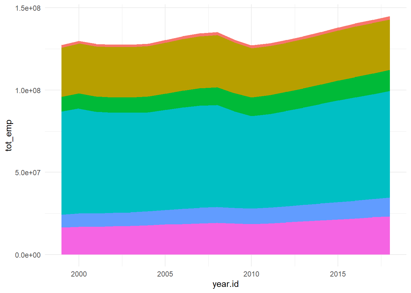

Creating the column emp_prct to show percentage share of each category for each year. For validation we can group it by year.id and then sum(emp_prct).
grouped_data2 <- grouped_data2 %>%
    dplyr::group_by(year.id) %>%
    dplyr::mutate(emp_prct = tot_emp * 1e2/sum(tot_emp),total = sum(tot_emp)) %>%
    dplyr::ungroup()

grouped_data <- grouped_data %>%
    dplyr::group_by(year.id) %>%
    dplyr::mutate(emp_prct = tot_emp * 1e2/sum(tot_emp),total = sum(tot_emp)) %>%
    dplyr::ungroup()
To put the data in perspective we can re-plot on as percentage of employment for each category over the years instead.
g <- grouped_data2 %>%
    ggplot2::ggplot(., aes(x = year.id, y = emp_prct, fill = category)) +
    geom_bar(stat = "identity")

g + theme_minimal() + theme(legend.position = "none") 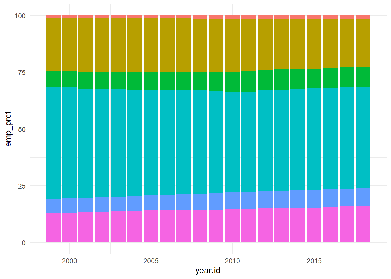

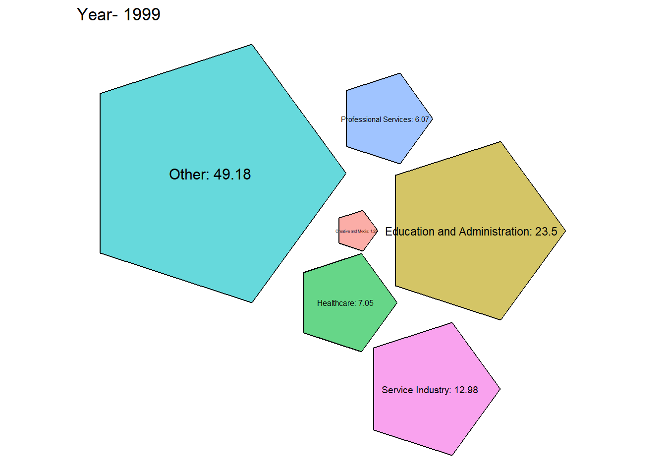
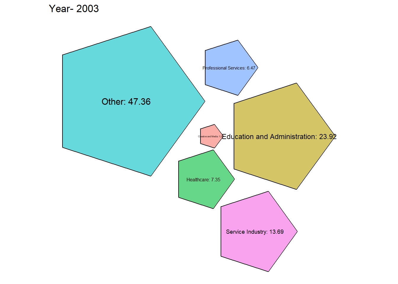
# Function to generate packed bubble plot for a specific year
generate_packed_bubble_plot <- function(year, grouped_data2) {
  data <- grouped_data2 %>%
    filter(year.id == year) %>%
    select(category, emp_prct)

  packing <- packcircles::circleProgressiveLayout(data$emp_prct, sizetype = 'area')

  data <- cbind(data, packing)

  dat.gg <- circleLayoutVertices(packing, npoints = 5)

  # Make the plot
  ggplot(data = dat.gg) +
    geom_polygon(aes(x, y, group = id, fill = as.factor(id)), colour = "black", alpha = 0.6) +
    geom_text(data = data, aes(x, y, size = emp_prct, label = paste0(category,": ",round(emp_prct, 2)))) +
    scale_size_continuous(range = c(1, 4)) +
    theme_void() +
    theme(legend.position = "none") +
    coord_equal() +
    labs(title = paste("Year-", year))
}
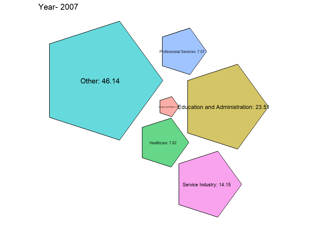
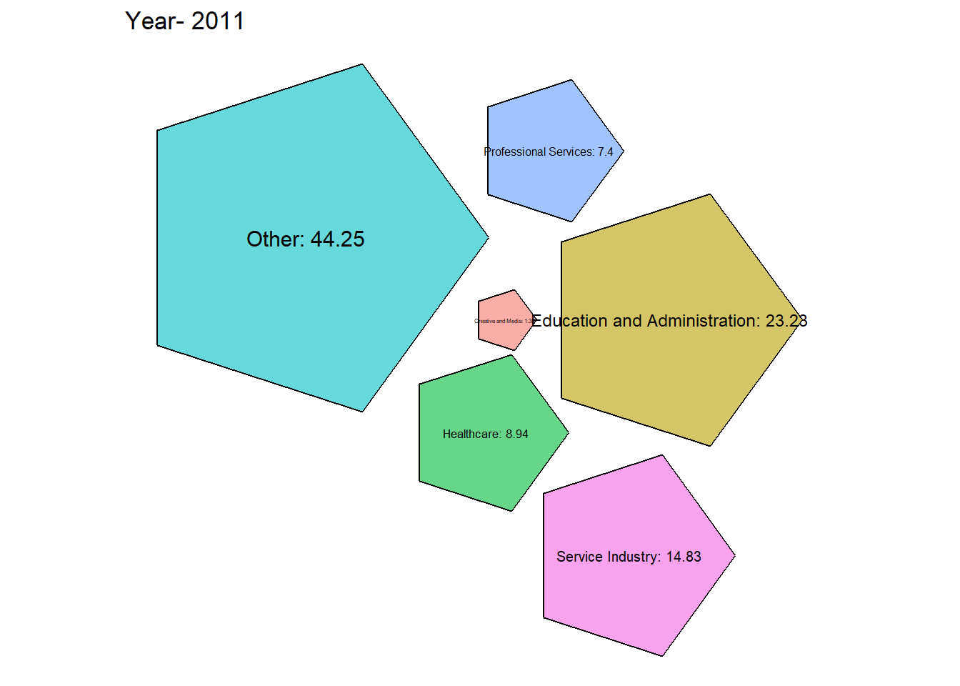

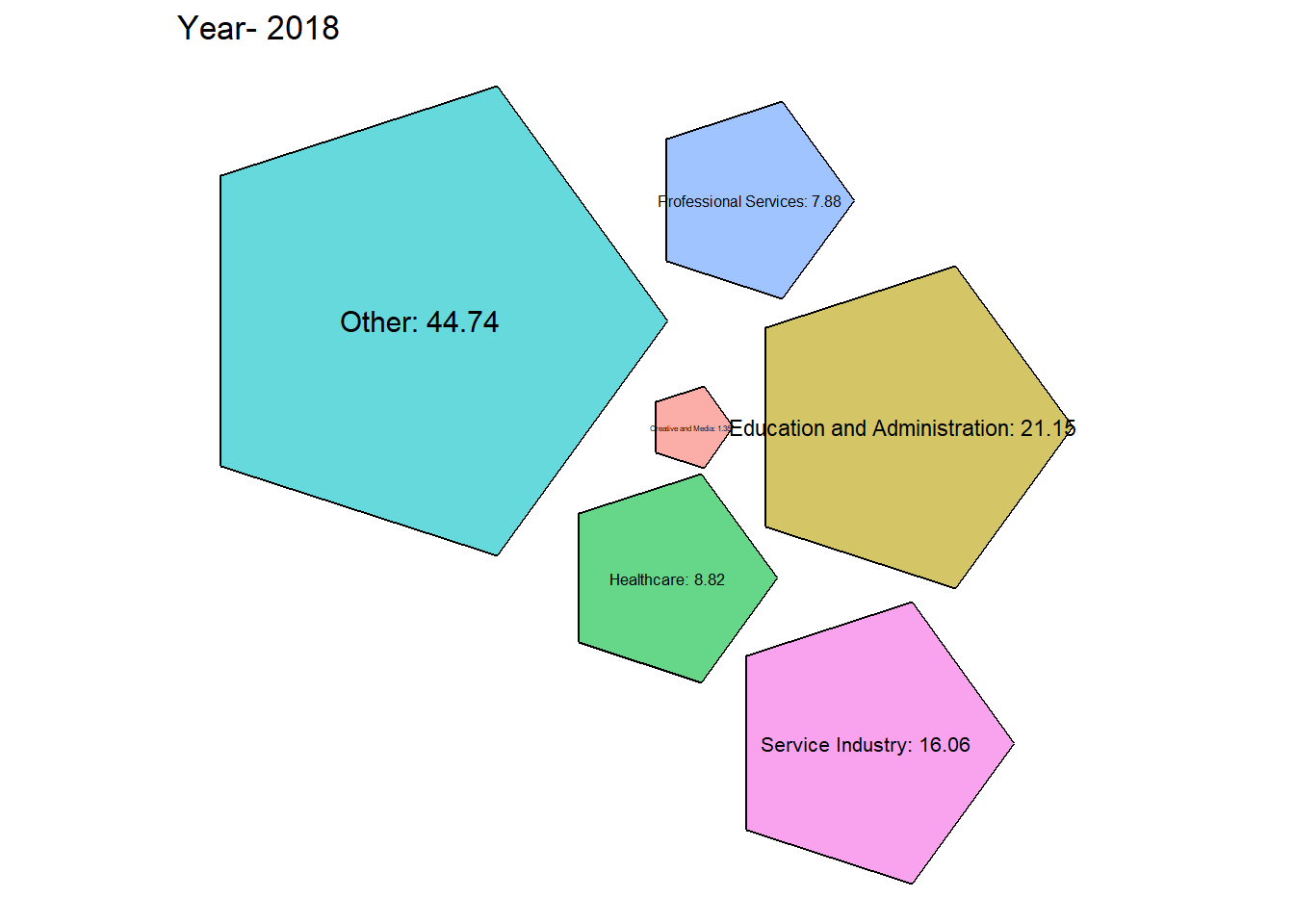
From the graph obtained we can see that there has been a steady growth in the service industry over the years along with Professional Services. Although Healthcare is one of the most important, it’s employment has always been \({< 10 \%}\) which is concerning.