library(tidyverse)
library(ggplot2)
knitr::opts_chunk$set(echo = TRUE, warning=FALSE, message=FALSE)
Challenge 5
challenge_5
air_bnb
Introduction to Visualization
Challenge Overview
Today’s challenge is to:
- read in a data set, and describe the data set using both words and any supporting information (e.g., tables, etc)
- tidy data (as needed, including sanity checks)
- mutate variables as needed (including sanity checks)
- create at least two univariate visualizations
- try to make them “publication” ready
- Explain why you choose the specific graph type
- Create at least one bivariate visualization
- try to make them “publication” ready
- Explain why you choose the specific graph type
R Graph Gallery is a good starting point for thinking about what information is conveyed in standard graph types, and includes example R code.
(be sure to only include the category tags for the data you use!)
Read in data
Read in one (or more) of the following datasets, using the correct R package and command.
- cereal.csv ⭐
- Total_cost_for_top_15_pathogens_2018.xlsx ⭐
- Australian Marriage ⭐⭐
- AB_NYC_2019.csv ⭐⭐⭐
- StateCounty2012.xls ⭐⭐⭐
- Public School Characteristics ⭐⭐⭐⭐
- USA Households ⭐⭐⭐⭐⭐
ab_nyc <- read.csv("_data/AB_NYC_2019.csv")
ab_nyc %>%  head()
id name host_id host_name
1 2539 Clean & quiet apt home by the park 2787 John
2 2595 Skylit Midtown Castle 2845 Jennifer
3 3647 THE VILLAGE OF HARLEM....NEW YORK ! 4632 Elisabeth
4 3831 Cozy Entire Floor of Brownstone 4869 LisaRoxanne
5 5022 Entire Apt: Spacious Studio/Loft by central park 7192 Laura
6 5099 Large Cozy 1 BR Apartment In Midtown East 7322 Chris
neighbourhood_group neighbourhood latitude longitude room_type price
1 Brooklyn Kensington 40.64749 -73.97237 Private room 149
2 Manhattan Midtown 40.75362 -73.98377 Entire home/apt 225
3 Manhattan Harlem 40.80902 -73.94190 Private room 150
4 Brooklyn Clinton Hill 40.68514 -73.95976 Entire home/apt 89
5 Manhattan East Harlem 40.79851 -73.94399 Entire home/apt 80
6 Manhattan Murray Hill 40.74767 -73.97500 Entire home/apt 200
minimum_nights number_of_reviews last_review reviews_per_month
1 1 9 2018-10-19 0.21
2 1 45 2019-05-21 0.38
3 3 0 NA
4 1 270 2019-07-05 4.64
5 10 9 2018-11-19 0.10
6 3 74 2019-06-22 0.59
calculated_host_listings_count availability_365
1 6 365
2 2 355
3 1 365
4 1 194
5 1 0
6 1 129Briefly describe the data
ab_nyc %>% colnames() [1] "id" "name"
[3] "host_id" "host_name"
[5] "neighbourhood_group" "neighbourhood"
[7] "latitude" "longitude"
[9] "room_type" "price"
[11] "minimum_nights" "number_of_reviews"
[13] "last_review" "reviews_per_month"
[15] "calculated_host_listings_count" "availability_365" This data represents the hotels and their prices in NYC. There are a total of 16 columns
ab_nyc$neighbourhood_group %>% unique()[1] "Brooklyn" "Manhattan" "Queens" "Staten Island"
[5] "Bronx" ab_nyc$room_type %>% unique()[1] "Private room" "Entire home/apt" "Shared room" ab_nyc$minimum_nights %>% unique() [1] 1 3 10 45 2 5 4 90 7 14 60 29 30 180 9
[16] 31 6 15 8 26 28 200 50 17 21 11 25 13 35 27
[31] 18 20 40 44 65 55 120 365 122 19 240 88 115 150 370
[46] 16 80 181 265 300 59 185 360 56 12 70 39 24 32 1000
[61] 110 270 22 75 250 62 23 1250 364 74 198 100 500 43 91
[76] 480 53 99 160 47 999 186 366 68 93 87 183 299 175 98
[91] 133 354 42 33 37 225 400 105 184 153 134 222 58 210 275
[106] 182 114 85 36There are three types of room - Private, Shared and Entire apartment. All the rooms are segregated into areas in NY. The minimum number of nights vary widely accross all the rentals.
Tidy Data (as needed)
Is your data already tidy, or is there work to be done? Be sure to anticipate your end result to provide a sanity check, and document your work here.
There are some missing values in some columns(For ex reviews_per_month). replace it with 0.
ab_nyc <- ab_nyc %>%  replace_na(list(reviews_per_month = 0))

ab_nyc <- ab_nyc %>%  filter(price>0)
Are there any variables that require mutation to be usable in your analysis stream? For example, do you need to calculate new values in order to graph them? Can string values be represented numerically? Do you need to turn any variables into factors and reorder for ease of graphics and visualization?
Document your work here.
Univariate Visualizations
ggplot(ab_nyc,aes(neighbourhood_group))+geom_bar()+labs(title = "Count of rentals in different neighbourhood groups")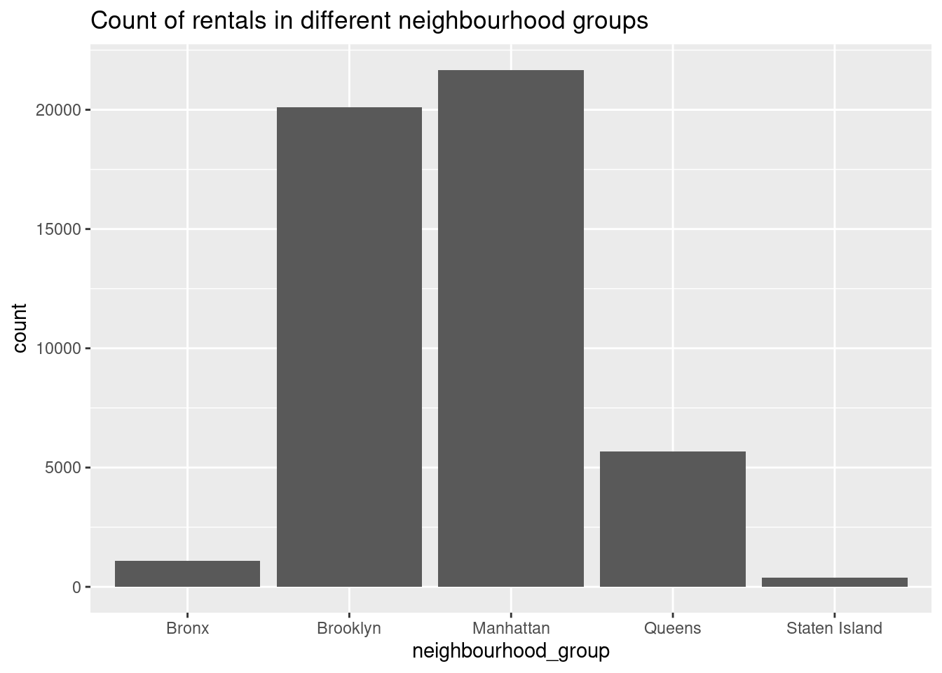
ggplot(ab_nyc,aes(room_type))+geom_bar()+labs(title = "Count of different type of rooms")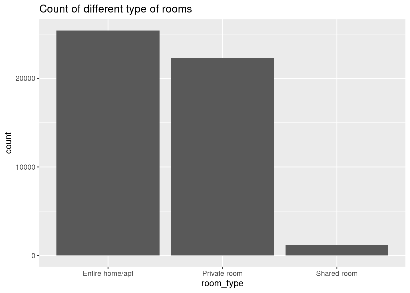
cheap_hotels <- ab_nyc %>% arrange(price) %>% filter(row_number()<1000)
ggplot(cheap_hotels,aes(price))+geom_histogram()+labs(title = "Price distribution of cheapest 1000 rooms")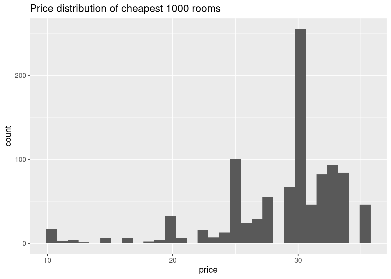
Bivariate Visualization(s)
ggplot(ab_nyc,aes(neighbourhood_group,price))+geom_point()+labs(title = "Distirbution of prices of hotels accross different neighbourhood_groups")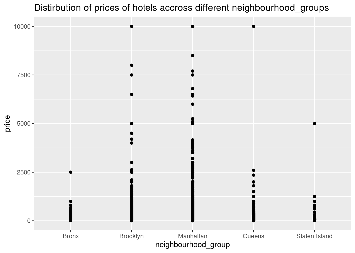
Any additional comments?