Challenge 8

challenge_8

railroads

snl

faostat

debt

Joining Data

Author

Aditya Salveru

Published

May 22, 2023

library(tidyverse)
library(ggplot2)

knitr::opts_chunk$set(echo = TRUE, warning=FALSE, message=FALSE)

Challenge Overview

Today’s challenge is to:

read in multiple data sets, and describe the data set using both words and any supporting information (e.g., tables, etc)
tidy data (as needed, including sanity checks)
mutate variables as needed (including sanity checks)
join two or more data sets and analyze some aspect of the joined data

(be sure to only include the category tags for the data you use!)

Read in data

Read in one (or more) of the following datasets, using the correct R package and command.

military marriages ⭐⭐
faostat ⭐⭐
railroads ⭐⭐⭐
fed_rate ⭐⭐⭐
debt ⭐⭐⭐
us_hh ⭐⭐⭐⭐
snl ⭐⭐⭐⭐⭐

Read the SNL data sets:

actors <- read.csv("_data/snl_actors.csv")
seasons <- read.csv("_data/snl_seasons.csv")
casts <- read.csv("_data/snl_casts.csv")

Briefly describe the data

Tidy Data (as needed)

dim(actors)

[1] 2306    4

head(actors,10)

              aid           url  type  gender
1   Kate McKinnon   /Cast/?KaMc  cast  female
2     Alex Moffat   /Cast/?AlMo  cast    male
3      Ego Nwodim   /Cast/?EgNw  cast unknown
4      Chris Redd   /Cast/?ChRe  cast    male
5  Kenan Thompson   /Cast/?KeTh  cast    male
6  Carey Mulligan /Guests/?3677 guest    andy
7  Marcus Mumford /Guests/?3679 guest    male
8     Aidy Bryant   /Cast/?AiBr  cast  female
9   Steve Higgins   /Crew/?StHi  crew    male
10      Mikey Day   /Cast/?MiDa  cast    male

dim(seasons)

[1] 46  5

head(seasons,10)

   sid year first_epid last_epid n_episodes
1    1 1975   19751011  19760731         24
2    2 1976   19760918  19770521         22
3    3 1977   19770924  19780520         20
4    4 1978   19781007  19790526         20
5    5 1979   19791013  19800524         20
6    6 1980   19801115  19810411         13
7    7 1981   19811003  19820522         20
8    8 1982   19820925  19830514         20
9    9 1983   19831008  19840512         19
10  10 1984   19841006  19850413         17

dim(casts)

[1] 614   8

head(casts,10)

                aid sid featured first_epid last_epid update_anchor n_episodes
1  A. Whitney Brown  11     True   19860222        NA         False          8
2  A. Whitney Brown  12     True         NA        NA         False         20
3  A. Whitney Brown  13     True         NA        NA         False         13
4  A. Whitney Brown  14     True         NA        NA         False         20
5  A. Whitney Brown  15     True         NA        NA         False         20
6  A. Whitney Brown  16     True         NA        NA         False         20
7      Alan Zweibel   5     True   19800409        NA         False          5
8    Sasheer Zamata  39     True   20140118        NA         False         11
9    Sasheer Zamata  40     True         NA        NA         False         21
10   Sasheer Zamata  41    False         NA        NA         False         21
   season_fraction
1        0.4444444
2        1.0000000
3        1.0000000
4        1.0000000
5        1.0000000
6        1.0000000
7        0.2500000
8        0.5238095
9        1.0000000
10       1.0000000

These three datasets include details about the casts, actors, and seasons of the TV show “Saturday Night Live.” These dataframes’ dimensions allow us to see that Saturday Night Live ran for 46 seasons and featured 2306 actors in total. The “casts” dataset includes information about the cast members’ appearances on the show, including specifics like their highlighted episodes, number of appearances, and other pertinent data. The “actors” dataset contains specific actor-related information. The “seasons” dataset contains details on each season of the show, including the premiere and finale episodes, the year that each season first aired, and the overall number of episodes that season had.

Check for NA values

colSums(is.na(actors))

   aid    url   type gender 
     0      0      0      0

colSums(is.na(seasons))

       sid       year first_epid  last_epid n_episodes 
         0          0          0          0          0

colSums(is.na(casts))

            aid             sid        featured      first_epid       last_epid 
              0               0               0             564             597 
  update_anchor      n_episodes season_fraction 
              0               0               0

There are not many missing values apart from the first and last epid in the casts table. We will clean it if necessary.

Join Data

actors_and_casts <- actors %>%
  inner_join(casts, by="aid")

actors_and_casts_and_seasons <- actors_and_casts %>%
  inner_join(seasons, by="sid")

colSums(is.na(actors_and_casts_and_seasons))

            aid             url            type          gender             sid 
              0               0               0               0               0 
       featured    first_epid.x     last_epid.x   update_anchor    n_episodes.x 
              0             564             597               0               0 
season_fraction            year    first_epid.y     last_epid.y    n_episodes.y 
              0               0               0               0               0

Ignore the columns with NA values

exclude_columns <- c("last_epid.x", "first_epid.x")

actors_and_casts_and_seasons <- actors_and_casts_and_seasons %>% 
  select(-one_of(exclude_columns))
head(actors_and_casts_and_seasons)

            aid         url type gender sid featured update_anchor n_episodes.x
1 Kate McKinnon /Cast/?KaMc cast female  37     True         False            5
2 Kate McKinnon /Cast/?KaMc cast female  38     True         False           21
3 Kate McKinnon /Cast/?KaMc cast female  39    False         False           21
4 Kate McKinnon /Cast/?KaMc cast female  40    False         False           21
5 Kate McKinnon /Cast/?KaMc cast female  41    False         False           21
6 Kate McKinnon /Cast/?KaMc cast female  42    False         False           21
  season_fraction year first_epid.y last_epid.y n_episodes.y
1       0.2272727 2011     20110924    20120519           22
2       1.0000000 2012     20120915    20130518           21
3       1.0000000 2013     20130928    20140517           21
4       1.0000000 2014     20140927    20150516           21
5       1.0000000 2015     20151003    20160521           21
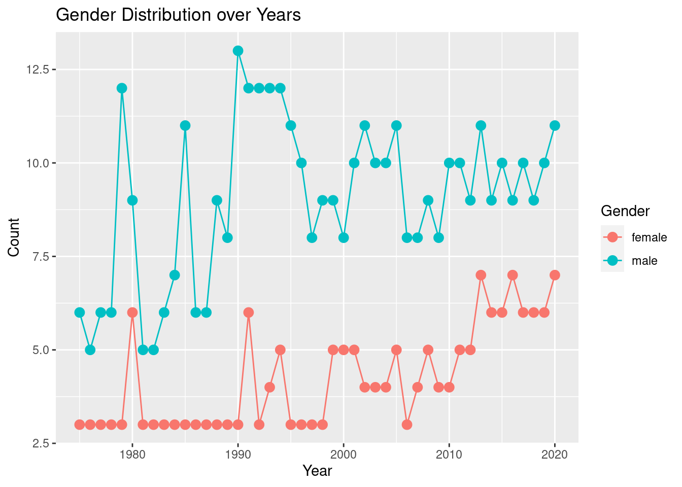
6       1.0000000 2016     20161001    20170520           21

From this joined data, we can plot the gender distribution over the years in the show

data <- actors_and_casts_and_seasons %>% 
  select(year, gender) %>%
  filter(gender == "male" | gender == "female")
# Create the line plot

# Count the number of occurrences of each gender per year
gender_counts <- data %>% group_by(year, gender) %>% summarise(count = n())

# Create the line plot
ggplot(gender_counts, aes(x = year, y = count, group = gender, color = gender)) +
  geom_line() +
  geom_point(size = 3) +
  labs(x = "Year", y = "Count", color = "Gender") +
  ggtitle("Gender Distribution over Years")