library(tidyverse)
library(ggplot2)
library(dplyr)
library(lubridate)
knitr::opts_chunk$set(echo = TRUE, warning=FALSE, message=FALSE)Challenge 7
challenge_7
air_bnb
Anirudh Lakkaraju
Visualizing Multiple Dimensions
Read in data
df <- read.csv("_data/AB_NYC_2019.csv")
head(df)
id name host_id host_name
1 2539 Clean & quiet apt home by the park 2787 John
2 2595 Skylit Midtown Castle 2845 Jennifer
3 3647 THE VILLAGE OF HARLEM....NEW YORK ! 4632 Elisabeth
4 3831 Cozy Entire Floor of Brownstone 4869 LisaRoxanne
5 5022 Entire Apt: Spacious Studio/Loft by central park 7192 Laura
6 5099 Large Cozy 1 BR Apartment In Midtown East 7322 Chris
neighbourhood_group neighbourhood latitude longitude room_type price
1 Brooklyn Kensington 40.64749 -73.97237 Private room 149
2 Manhattan Midtown 40.75362 -73.98377 Entire home/apt 225
3 Manhattan Harlem 40.80902 -73.94190 Private room 150
4 Brooklyn Clinton Hill 40.68514 -73.95976 Entire home/apt 89
5 Manhattan East Harlem 40.79851 -73.94399 Entire home/apt 80
6 Manhattan Murray Hill 40.74767 -73.97500 Entire home/apt 200
minimum_nights number_of_reviews last_review reviews_per_month
1 1 9 2018-10-19 0.21
2 1 45 2019-05-21 0.38
3 3 0 NA
4 1 270 2019-07-05 4.64
5 10 9 2018-11-19 0.10
6 3 74 2019-06-22 0.59
calculated_host_listings_count availability_365
1 6 365
2 2 355
3 1 365
4 1 194
5 1 0
6 1 129dim(df)[1] 48895 16summary(df) id name host_id host_name
Min. : 2539 Length:48895 Min. : 2438 Length:48895
1st Qu.: 9471945 Class :character 1st Qu.: 7822033 Class :character
Median :19677284 Mode :character Median : 30793816 Mode :character
Mean :19017143 Mean : 67620011
3rd Qu.:29152178 3rd Qu.:107434423
Max. :36487245 Max. :274321313
neighbourhood_group neighbourhood latitude longitude
Length:48895 Length:48895 Min. :40.50 Min. :-74.24
Class :character Class :character 1st Qu.:40.69 1st Qu.:-73.98
Mode :character Mode :character Median :40.72 Median :-73.96
Mean :40.73 Mean :-73.95
3rd Qu.:40.76 3rd Qu.:-73.94
Max. :40.91 Max. :-73.71
room_type price minimum_nights number_of_reviews
Length:48895 Min. : 0.0 Min. : 1.00 Min. : 0.00
Class :character 1st Qu.: 69.0 1st Qu.: 1.00 1st Qu.: 1.00
Mode :character Median : 106.0 Median : 3.00 Median : 5.00
Mean : 152.7 Mean : 7.03 Mean : 23.27
3rd Qu.: 175.0 3rd Qu.: 5.00 3rd Qu.: 24.00
Max. :10000.0 Max. :1250.00 Max. :629.00
last_review reviews_per_month calculated_host_listings_count
Length:48895 Min. : 0.010 Min. : 1.000
Class :character 1st Qu.: 0.190 1st Qu.: 1.000
Mode :character Median : 0.720 Median : 1.000
Mean : 1.373 Mean : 7.144
3rd Qu.: 2.020 3rd Qu.: 2.000
Max. :58.500 Max. :327.000
NA's :10052
availability_365
Min. : 0.0
1st Qu.: 0.0
Median : 45.0
Mean :112.8
3rd Qu.:227.0
Max. :365.0
Briefly describe the data
The dataset contains information about approximately 49,000 rental properties available on Airbnb in New York City during 2019. Each entry represents a unique rental unit and includes 16 different variables, including details like the unit’s ID, name, location, host ID and name, room type, price, minimum nights required for booking, number of reviews, date of the last review, average monthly reviews, calculated count of host listings on Airbnb, and availability.
str(df)'data.frame': 48895 obs. of 16 variables:
$ id : int 2539 2595 3647 3831 5022 5099 5121 5178 5203 5238 ...
$ name : chr "Clean & quiet apt home by the park" "Skylit Midtown Castle" "THE VILLAGE OF HARLEM....NEW YORK !" "Cozy Entire Floor of Brownstone" ...
$ host_id : int 2787 2845 4632 4869 7192 7322 7356 8967 7490 7549 ...
$ host_name : chr "John" "Jennifer" "Elisabeth" "LisaRoxanne" ...
$ neighbourhood_group : chr "Brooklyn" "Manhattan" "Manhattan" "Brooklyn" ...
$ neighbourhood : chr "Kensington" "Midtown" "Harlem" "Clinton Hill" ...
$ latitude : num 40.6 40.8 40.8 40.7 40.8 ...
$ longitude : num -74 -74 -73.9 -74 -73.9 ...
$ room_type : chr "Private room" "Entire home/apt" "Private room" "Entire home/apt" ...
$ price : int 149 225 150 89 80 200 60 79 79 150 ...
$ minimum_nights : int 1 1 3 1 10 3 45 2 2 1 ...
$ number_of_reviews : int 9 45 0 270 9 74 49 430 118 160 ...
$ last_review : chr "2018-10-19" "2019-05-21" "" "2019-07-05" ...
$ reviews_per_month : num 0.21 0.38 NA 4.64 0.1 0.59 0.4 3.47 0.99 1.33 ...
$ calculated_host_listings_count: int 6 2 1 1 1 1 1 1 1 4 ...
$ availability_365 : int 365 355 365 194 0 129 0 220 0 188 ...Tidy Data (as needed)
df <- na.omit(df)
df <- df %>% mutate(high_price = ifelse(price > 500, "High", "Low"))
Visualization with Multiple Dimensions
Univariate visualization using histogram
library(ggplot2)
ggplot(df, aes(x=price)) +
  geom_histogram(binwidth=25, color="blue", fill="blue") +
  labs(title="Distribution of Price", x="Price", y="Frequency")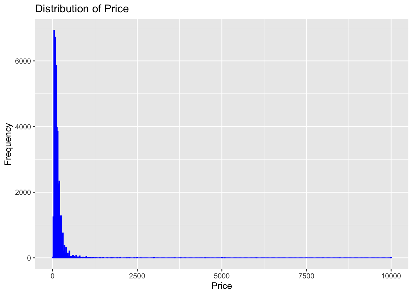
Bi-variate Visualizations :
The initial scatterplot illustrates the correlation between price and reviews_per_month within the complete dataset. The plot is created using the ggplot function, with the aes function specifying the variables for the x and y axes. Data points are then added to the plot using geom_point, and the title and axis labels are defined using labs.
ggplot(df, aes(x=price, y=reviews_per_month)) +
  geom_point(alpha=0.46, color="red") +
  labs(title="Monthly Price vs Reviews", x="Price", y="Reviews per Month")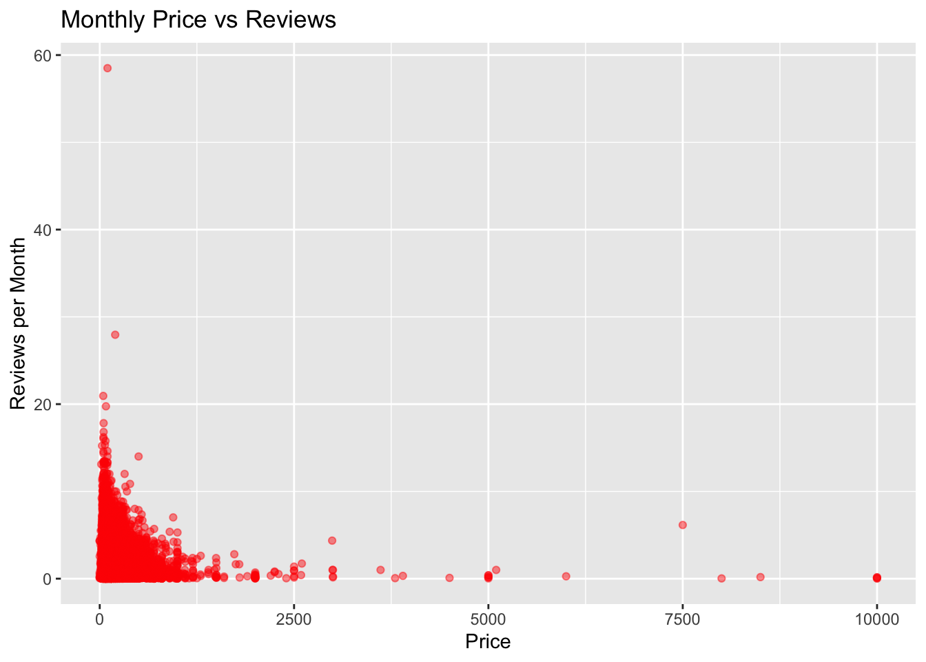
ggplot(df, aes(x=price, y=reviews_per_month)) +
  geom_point(alpha=0.5, color="red") +
  labs(title="Price vs Reviews per Month by City", x="Price", y="Reviews per Month") +
  facet_wrap(~ neighbourhood_group, scales="free")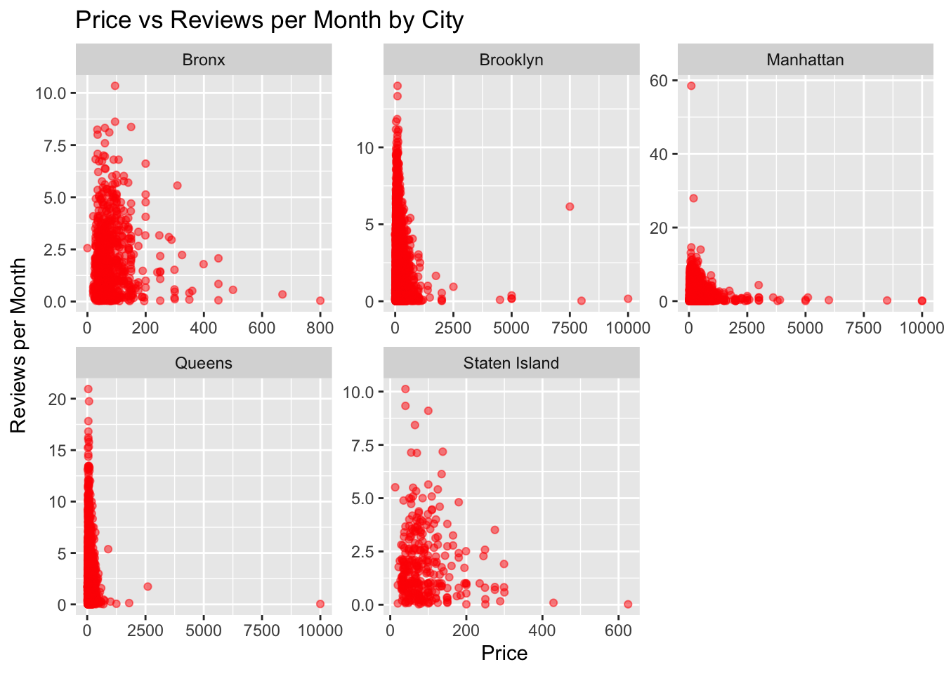
I opted for a scatter plot to visually represent the correlation between price and reviews per month across different cities. This choice was made because a scatter plot effectively displays individual data points as well as the general trend in the data. By utilizing this plot, we can observe whether there is a connection between price and reviews per month, as well as identify any outliers or patterns within the data. Additionally, the use of distinct colors to represent each city aids in distinguishing the data points associated with each specific location.