Read in a data set, and describe the data set using both words and any supporting information (e.g., tables, etc)
Tidy data & mutate variables as needed (including sanity checks)
Recreate at least two graphs from previous exercises, but introduce at least one additional dimension that you omitted before using ggplot functionality (color, shape, line, facet, etc) The goal is not to create unneeded chart ink (Tufte), but to concisely capture variation in additional dimensions that were collapsed in your earlier 2 or 3 dimensional graphs.
If you haven’t tried in previous weeks, work this week to make your graphs “publication” ready with titles, captions, and pretty axis labels and other viewer-friendly features
Read in data
Code
#read in the data set, rawlibrary(readr)raw_airbnb <-read_csv("_data/AB_NYC_2019.csv")raw_airbnb
Briefly describe the data
I analyzed this data set in Challenge 5. It describes around 49k Airbnb property listings in NYC boroughs for the year of 2019. Each property listing includes information about geographical location (neighborhood borough/name, latitude/longitude), rental type (entire home/apt, private room, or shared room), price, minimum nights stayed, reviews (last review, total number & per month) and how many days available in 2019. In the next code chunk, I tidied up the data so I can graph price by NYC borough later on.
Code
#summary of data set statisticsprint(summarytools::dfSummary(raw_airbnb,varnumbers =FALSE,plain.ascii =FALSE, style ="grid", graph.magnif =0.70, valid.col =FALSE),method ='render',table.classes ='table-condensed')
Data Frame Summary
raw_airbnb
Dimensions: 48895 x 16
Duplicates: 0
Variable
Stats / Values
Freqs (% of Valid)
Graph
Missing
id [numeric]
Mean (sd) : 19017143 (10983108)
min ≤ med ≤ max:
2539 ≤ 19677284 ≤ 36487245
IQR (CV) : 19680234 (0.6)
48895 distinct values
0 (0.0%)
name [character]
1. Hillside Hotel
2. Home away from home
3. New york Multi-unit build
4. Brooklyn Apartment
5. Loft Suite @ The Box Hous
6. Private Room
7. Artsy Private BR in Fort
8. Private room
9. Beautiful Brooklyn Browns
10. Cozy Brooklyn Apartment
[ 47884 others ]
18
(
0.0%
)
17
(
0.0%
)
16
(
0.0%
)
12
(
0.0%
)
11
(
0.0%
)
11
(
0.0%
)
10
(
0.0%
)
10
(
0.0%
)
8
(
0.0%
)
8
(
0.0%
)
48758
(
99.8%
)
16 (0.0%)
host_id [numeric]
Mean (sd) : 67620011 (78610967)
min ≤ med ≤ max:
2438 ≤ 30793816 ≤ 274321313
IQR (CV) : 99612390 (1.2)
37457 distinct values
0 (0.0%)
host_name [character]
1. Michael
2. David
3. Sonder (NYC)
4. John
5. Alex
6. Blueground
7. Sarah
8. Daniel
9. Jessica
10. Maria
[ 11442 others ]
417
(
0.9%
)
403
(
0.8%
)
327
(
0.7%
)
294
(
0.6%
)
279
(
0.6%
)
232
(
0.5%
)
227
(
0.5%
)
226
(
0.5%
)
205
(
0.4%
)
204
(
0.4%
)
46060
(
94.2%
)
21 (0.0%)
neighbourhood_group [character]
1. Bronx
2. Brooklyn
3. Manhattan
4. Queens
5. Staten Island
1091
(
2.2%
)
20104
(
41.1%
)
21661
(
44.3%
)
5666
(
11.6%
)
373
(
0.8%
)
0 (0.0%)
neighbourhood [character]
1. Williamsburg
2. Bedford-Stuyvesant
3. Harlem
4. Bushwick
5. Upper West Side
6. Hell's Kitchen
7. East Village
8. Upper East Side
9. Crown Heights
10. Midtown
[ 211 others ]
3920
(
8.0%
)
3714
(
7.6%
)
2658
(
5.4%
)
2465
(
5.0%
)
1971
(
4.0%
)
1958
(
4.0%
)
1853
(
3.8%
)
1798
(
3.7%
)
1564
(
3.2%
)
1545
(
3.2%
)
25449
(
52.0%
)
0 (0.0%)
latitude [numeric]
Mean (sd) : 40.7 (0.1)
min ≤ med ≤ max:
40.5 ≤ 40.7 ≤ 40.9
IQR (CV) : 0.1 (0)
19048 distinct values
0 (0.0%)
longitude [numeric]
Mean (sd) : -74 (0)
min ≤ med ≤ max:
-74.2 ≤ -74 ≤ -73.7
IQR (CV) : 0 (0)
14718 distinct values
0 (0.0%)
room_type [character]
1. Entire home/apt
2. Private room
3. Shared room
25409
(
52.0%
)
22326
(
45.7%
)
1160
(
2.4%
)
0 (0.0%)
price [numeric]
Mean (sd) : 152.7 (240.2)
min ≤ med ≤ max:
0 ≤ 106 ≤ 10000
IQR (CV) : 106 (1.6)
674 distinct values
0 (0.0%)
minimum_nights [numeric]
Mean (sd) : 7 (20.5)
min ≤ med ≤ max:
1 ≤ 3 ≤ 1250
IQR (CV) : 4 (2.9)
109 distinct values
0 (0.0%)
number_of_reviews [numeric]
Mean (sd) : 23.3 (44.6)
min ≤ med ≤ max:
0 ≤ 5 ≤ 629
IQR (CV) : 23 (1.9)
394 distinct values
0 (0.0%)
last_review [Date]
min : 2011-03-28
med : 2019-05-19
max : 2019-07-08
range : 8y 3m 10d
1764 distinct values
10052 (20.6%)
reviews_per_month [numeric]
Mean (sd) : 1.4 (1.7)
min ≤ med ≤ max:
0 ≤ 0.7 ≤ 58.5
IQR (CV) : 1.8 (1.2)
937 distinct values
10052 (20.6%)
calculated_host_listings_count [numeric]
Mean (sd) : 7.1 (33)
min ≤ med ≤ max:
1 ≤ 1 ≤ 327
IQR (CV) : 1 (4.6)
47 distinct values
0 (0.0%)
availability_365 [numeric]
Mean (sd) : 112.8 (131.6)
min ≤ med ≤ max:
0 ≤ 45 ≤ 365
IQR (CV) : 227 (1.2)
366 distinct values
0 (0.0%)
Generated by summarytools 1.0.1 (R version 4.2.2) 2023-04-17
Code
#created new data table in order to graph borough by price segmented by room typetidy_Airbnb <- raw_airbnb %>%filter(room_type =="Shared room"| room_type =="Entire home/apt"| room_type =="Private room") %>%group_by(neighbourhood_group, room_type) %>%summarise(mean_price=mean(price))tidy_Airbnb
Visualization with Multiple Dimensions
In my previous challenge, I created univariate and bivariate visualizations of this data which analyzed price, neighborhood borough, and room type. Today, I will revisit these graphs and create new visualizations which introduce at least one additional dimension.
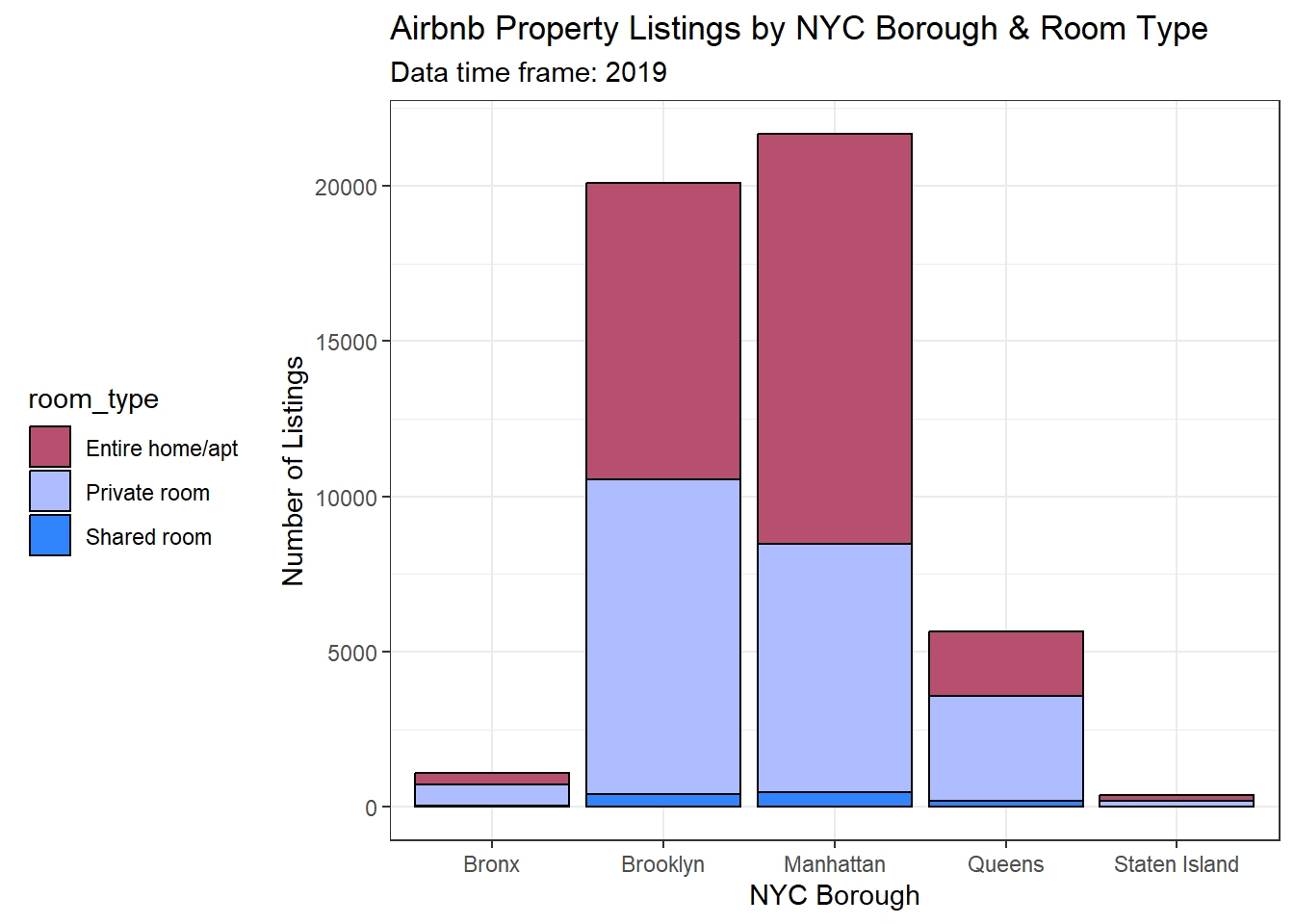
See the first graph below. It shows number of property listings by neighborhood borough segmented by room type. Key takeaways:
Manhattan and Brooklyn have the most listings while Staten Island and Bronx have the least number of listings
The most common room type for the majority of listings is entire home/apartment with shared room being the least common
Overall, Manhattan has the most listings and highest ratio of entire home/apartment to other room types
Code
#bar graph to visualize number of listings by borough and room typecbbPalette <-c("#B74F6F", "#ADBDFF", "#3185FC")bar_Airbnb <-ggplot(raw_airbnb, aes(neighbourhood_group, fill = room_type, na.rm =TRUE)) +geom_bar(stat ="count", colour="black") +labs(title ="Airbnb Property Listings by NYC Borough & Room Type", x ="NYC Borough", y ="Number of Listings", subtitle ="Data time frame: 2019") +scale_fill_discrete(name ="Room Type") +theme_bw() +theme(legend.position ="left") +scale_fill_manual(values=cbbPalette)bar_Airbnb
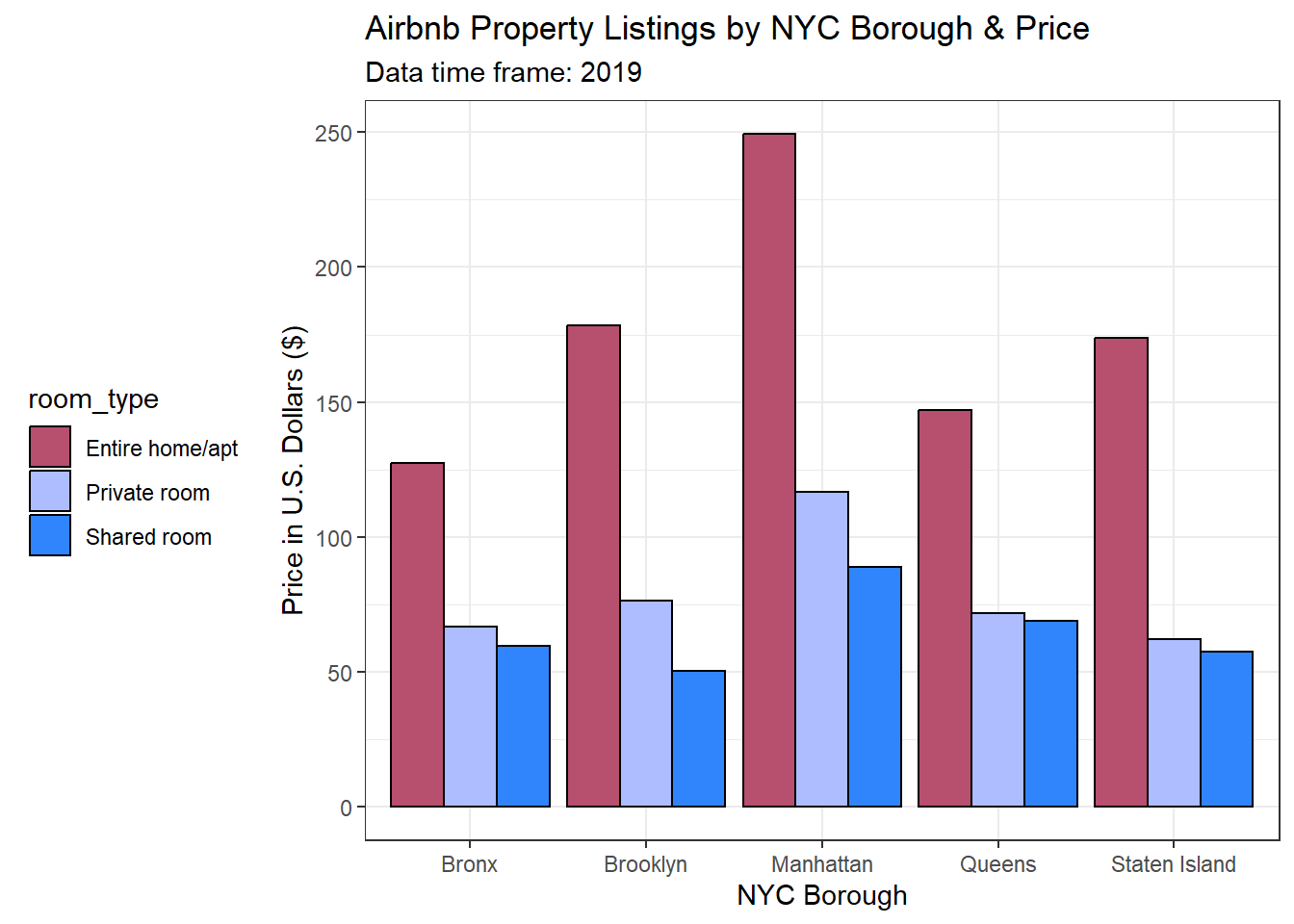
At a high level, it is clear that Manhattan has the most listings, but it is the most expensive? The graph below answers that question, yes! Not only are it’s property prices the most expensive on average, but the entire home/apartment price is the highest priced of all the NYC boroughs. For NYC, this result makes sense since it is a highly sought after neighborhood.
Code
#bar graph to visualize price of listings by borough and room typeprice_Airbnb <- tidy_Airbnb %>%ggplot(tidy_airbnb, mapping =aes(neighbourhood_group, mean_price, fill = room_type)) +geom_bar(position ="dodge", stat ="identity", colour="black") +labs(title ="Airbnb Property Listings by NYC Borough & Price", x ="NYC Borough", y ="Price in U.S. Dollars ($)", subtitle ="Data time frame: 2019") +scale_fill_discrete(name ="Room Type") +theme_bw() +theme(legend.position ="left") +scale_fill_manual(values=cbbPalette)price_Airbnb
Source Code
---title: "Challenge 7 - Airbnb Listings"author: "Megan Galarneau"description: "Visualizing Multiple Dimensions"date: "04/17/2023"format: html: df-print: paged toc: true code-fold: true code-copy: true code-tools: true css: "style.css"categories: - challenge_7 - air_bnb - Megan Galarneau---```{r}#| label: setup#| warning: false#| message: falselibrary(tidyverse)library(ggplot2)library(dplyr)library(lubridate)library(patchwork)knitr::opts_chunk$set(echo =TRUE, warning=FALSE, message=FALSE)```## Challenge OverviewToday's challenge is to:1) Read in a data set, and describe the data set using both words and any supporting information (e.g., tables, etc)2) Tidy data & mutate variables as needed (including sanity checks)3) Recreate at least two graphs from previous exercises, but introduce at least one additional dimension that you omitted before using ggplot functionality (color, shape, line, facet, etc) The goal is not to create unneeded [chart ink (Tufte)](https://www.edwardtufte.com/tufte/), but to concisely capture variation in additional dimensions that were collapsed in your earlier 2 or 3 dimensional graphs.5) If you haven't tried in previous weeks, work this week to make your graphs "publication" ready with titles, captions, and pretty axis labels and other viewer-friendly features## Read in data```{r}#read in the data set, rawlibrary(readr)raw_airbnb <-read_csv("_data/AB_NYC_2019.csv")raw_airbnb```### Briefly describe the dataI analyzed this data set in Challenge 5. It describes around 49k Airbnb property listings in NYC boroughs for the year of 2019. Each property listing includes information about geographical location (neighborhood borough/name, latitude/longitude), rental type (entire home/apt, private room, or shared room), price, minimum nights stayed, reviews (last review, total number & per month) and how many days available in 2019. In the next code chunk, I tidied up the data so I can graph price by NYC borough later on.```{r}#summary of data set statisticsprint(summarytools::dfSummary(raw_airbnb,varnumbers =FALSE,plain.ascii =FALSE, style ="grid", graph.magnif =0.70, valid.col =FALSE),method ='render',table.classes ='table-condensed')``````{r}#created new data table in order to graph borough by price segmented by room typetidy_Airbnb <- raw_airbnb %>%filter(room_type =="Shared room"| room_type =="Entire home/apt"| room_type =="Private room") %>%group_by(neighbourhood_group, room_type) %>%summarise(mean_price=mean(price))tidy_Airbnb```## Visualization with Multiple DimensionsIn my previous challenge, I created univariate and bivariate visualizations of this data which analyzed price, neighborhood borough, and room type. Today, I will revisit these graphs and create new visualizations which introduce at least one additional dimension.See the first graph below. It shows number of property listings by neighborhood borough segmented by room type. Key takeaways:- Manhattan and Brooklyn have the most listings while Staten Island and Bronx have the least number of listings- The most common room type for the majority of listings is entire home/apartment with shared room being the least common- Overall, Manhattan has the most listings and highest ratio of entire home/apartment to other room types```{r}#bar graph to visualize number of listings by borough and room typecbbPalette <-c("#B74F6F", "#ADBDFF", "#3185FC")bar_Airbnb <-ggplot(raw_airbnb, aes(neighbourhood_group, fill = room_type, na.rm =TRUE)) +geom_bar(stat ="count", colour="black") +labs(title ="Airbnb Property Listings by NYC Borough & Room Type", x ="NYC Borough", y ="Number of Listings", subtitle ="Data time frame: 2019") +scale_fill_discrete(name ="Room Type") +theme_bw() +theme(legend.position ="left") +scale_fill_manual(values=cbbPalette)bar_Airbnb```At a high level, it is clear that Manhattan has the most listings, but it is the most expensive? The graph below answers that question, yes! Not only are it's property prices the most expensive on average, but the entire home/apartment price is the highest priced of all the NYC boroughs. For NYC, this result makes sense since it is a highly sought after neighborhood.```{r}#bar graph to visualize price of listings by borough and room typeprice_Airbnb <- tidy_Airbnb %>%ggplot(tidy_airbnb, mapping =aes(neighbourhood_group, mean_price, fill = room_type)) +geom_bar(position ="dodge", stat ="identity", colour="black") +labs(title ="Airbnb Property Listings by NYC Borough & Price", x ="NYC Borough", y ="Price in U.S. Dollars ($)", subtitle ="Data time frame: 2019") +scale_fill_discrete(name ="Room Type") +theme_bw() +theme(legend.position ="left") +scale_fill_manual(values=cbbPalette)price_Airbnb```