Are there any variables that require mutation to be usable in your analysis stream? For example, do you need to calculate new values in order to graph them? Can string values be represented numerically? Do you need to turn any variables into factors and reorder for ease of graphics and visualization?
Document your work here.
Join Data
Be sure to include a sanity check, and double-check that case count is correct
# A tibble: 2,764 × 14
aid gender type url sid featu…¹ year season_f…² season_l…³ actor_fi…⁴
<chr> <chr> <chr> <chr> <dbl> <lgl> <dbl> <date> <date> <date>
1 Chev… male cast /Cas… 1 FALSE 1975 1975-10-11 1976-07-31 NA
2 Dan … male cast /Cas… 1 FALSE 1975 1975-10-11 1976-07-31 NA
3 Garr… male cast /Cas… 1 FALSE 1975 1975-10-11 1976-07-31 NA
4 John… male cast /Cas… 1 FALSE 1975 1975-10-11 1976-07-31 NA
5 Mich… male cast /Cas… 1 FALSE 1975 1975-10-11 1976-07-31 NA
6 Jane… female cast /Cas… 1 FALSE 1975 1975-10-11 1976-07-31 NA
7 Lara… female cast /Cas… 1 FALSE 1975 1975-10-11 1976-07-31 NA
8 Gild… female cast /Cas… 1 FALSE 1975 1975-10-11 1976-07-31 NA
9 Geor… male cast /Cas… 1 FALSE 1975 1975-10-11 1976-07-31 NA
10 Bill… male cast /Cas… 2 FALSE 1976 1976-09-18 1977-05-21 1977-01-15
# … with 2,754 more rows, 4 more variables: actor_last_epid <date>,
# update_anchor <lgl>, n_actor_episodes <dbl>, season_fraction <dbl>, and
# abbreviated variable names ¹featured, ²season_first_epid,
# ³season_last_epid, ⁴actor_first_epid
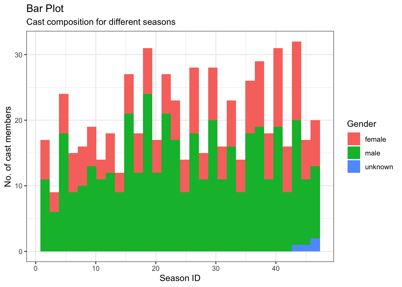
Visualisation
actors_merged %>%ggplot(aes(sid, fill = gender)) +geom_histogram(bins=30) +theme_bw() +labs(title ="Bar Plot", subtitle ="Cast composition for different seasons", y ="No. of cast members", x ="Season ID", fill ="Gender")
Source Code
---title: "Challenge 8 Paritosh"author: "Paritosh G"description: "Joining Data"date: "05/29/2023"format: html: toc: true code-copy: true code-tools: truecategories: - challenge_8 - railroads - snl - faostat - debt---```{r}library(tidyverse)library(ggplot2)knitr::opts_chunk$set(echo =TRUE, warning=FALSE, message=FALSE)```## Challenge OverviewToday's challenge is to:1) read in multiple data sets, and describe the data set using both words and any supporting information (e.g., tables, etc)2) tidy data (as needed, including sanity checks)3) mutate variables as needed (including sanity checks)4) join two or more data sets and analyze some aspect of the joined data(be sure to only include the category tags for the data you use!)## Read in 3 datasets.Read in one (or more) of the following datasets, using the correct R package and command.- snl ⭐⭐⭐⭐⭐```{r}actors <-read_csv("_data/snl_actors.csv")casts <-read_csv("_data/snl_casts.csv")seasons <-read_csv("_data/snl_seasons.csv")```### Briefly describe the data```{r}colnames(actors)``````{r}colnames(casts)``````{r}colnames(seasons)```## Tidy Data (as needed)Is your data already tidy, or is there work to be done? Be sure to anticipate your end result to provide a sanity check, and document your work here.```{r}casts <- casts %>%mutate(first_epid =ymd(first_epid), last_epid =ymd(last_epid))``````{r}seasons <- seasons %>%mutate(first_epid =ymd(first_epid), last_epid =ymd(last_epid))```Are there any variables that require mutation to be usable in your analysis stream? For example, do you need to calculate new values in order to graph them? Can string values be represented numerically? Do you need to turn any variables into factors and reorder for ease of graphics and visualization?Document your work here.## Join DataBe sure to include a sanity check, and double-check that case count is correct```{r}actors_merged <- actors %>%left_join(casts, by ="aid") %>%rename("actor_first_epid"="first_epid", "actor_last_epid"="last_epid", "n_actor_episodes"="n_episodes") %>%left_join(seasons, by ="sid") %>%rename("season_first_epid"="first_epid", "season_last_epid"="last_epid") %>%select(1, 4, 3, 2, 5, 6, 12:14, 7:11) %>%arrange(season_first_epid) actors_merged```## Visualisation```{r warning=FALSE}actors_merged %>%ggplot(aes(sid, fill = gender)) +geom_histogram(bins=30) +theme_bw() +labs(title ="Bar Plot", subtitle ="Cast composition for different seasons", y ="No. of cast members", x ="Season ID", fill ="Gender")```