Describing Global Poultry Production Data

Code

library(tidyverse)

knitr::opts_chunk$set(echo = TRUE, warning=FALSE, message=FALSE)

setwd("/Users/dirichiumunna/Documents/DACS601/GITHUB/dacss601_spring2023/posts/_data")

Challenge Overview

This blog post attempts to make descriptive sense of the data set titled “bird”. We begin by reading in the data, then generating an overview description of the data and some subsequent visualization.

Reading in the data set

Code

#using the readr package
library(readr)

birdset <- read.csv("/Users/dirichiumunna/Documents/DACS601/GITHUB/dacss601_spring2023/posts/_data/birds.csv")

By simply loading the data, it is clear that there are 14 variables and 30,977 observations from the information contained in the environment window. Next, I will check the variable and browse through the data just to get a sense of what the data is about.

Checking Data Context

Code

library(dplyr)
#getting basic descriptions for the data
  dim(birdset)

[1] 30977    14

We have discovered that there are 14 variables in the data set named: Domain Code, Domain, Area Code, Area, Element Code, Element, Item Code, Item, Year Code, Year, Unit, Value, Flag, and Flag Description. When we take a deeper dive into the content of the variables and we can see that this data provides information about countries’ birds production for a number of years, with each row containing the data per country, per year. Next, we narrow down some important variables.

Code

#narrow down useful variables
  birdset %>% select(Year, Area, Item, Value, Flag.Description, Domain)  %>%  
  summary()

      Year          Area               Item               Value         
 Min.   :1961   Length:30977       Length:30977       Min.   :       0  
 1st Qu.:1976   Class :character   Class :character   1st Qu.:     171  
 Median :1992   Mode  :character   Mode  :character   Median :    1800  
 Mean   :1991                                         Mean   :   99411  
 3rd Qu.:2005                                         3rd Qu.:   15404  
 Max.   :2018                                         Max.   :23707134  
                                                      NA's   :1036      
 Flag.Description      Domain         
 Length:30977       Length:30977      
 Class :character   Class :character  
 Mode  :character   Mode  :character  
                                      
                                      
                                      
                                      

Code

#separate count for Area and Item because they are character variables
  birdset %>%
  summarise(n_distinct(Area))

  n_distinct(Area)
1              248

Code

  table(birdset$Item)

              Chickens                  Ducks Geese and guinea fowls 
                 13074                   6909                   4136 
  Pigeons, other birds                Turkeys 
                  1165                   5693 

We have now been provided more data about the selected variables. The dataset contains values for years 1961 to 2018, for 248 countries, with 6 poultry categories (Chicken, ducks, Geese and Guinea fowls, Turkeys and other birds), with the data retrieved from 6 sources linked to the FAO (Food and agriculture organization). The domain variable tells us that the data set is restricted to live animals; while the values shows the measurement of production. Now, we have gotten a clearer picture of the dataset which shows the amount of poultry production by different countries.

Visualization

Next, we want to see a little bit of the visualization for this dataset. Specifically, we will look at which birds are globally produced more and what countries have the highest number of production. First we create a bar plot showing the most produced bird type:

Code

library(ggplot2)
  ggplot(data = birdset) +
  geom_col(mapping = aes(x = Item, y = Value)) +
  labs(title = "Bird Production by Type", x = "Bird Type", y = "Number Produced")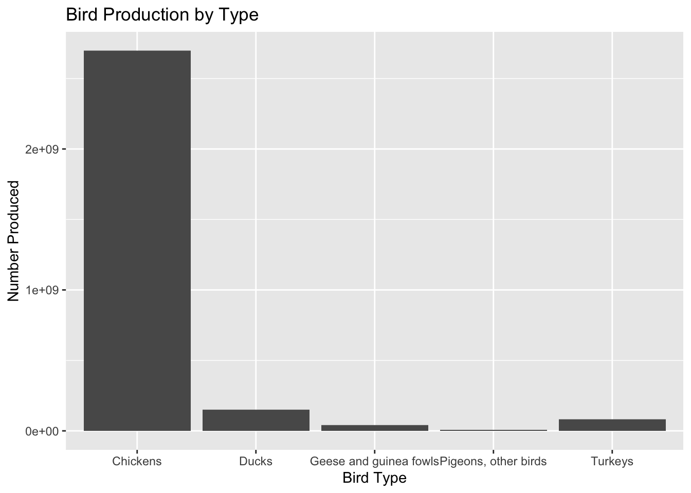

Next, we will look at countries with the highest production of bird type, specifically,Chicken.

Code

library(dplyr)

#create a new vector with the specifications for top country by value
top_countries <- birdset %>%
  filter(Item == "Chickens") %>%
  group_by(Area) %>%
  summarise(total_value = sum(Value)) %>%
  arrange(desc(total_value)) %>%
  slice(1:5)


#create another vector to filter by top country and chicken
filtered_data <- birdset %>%
  filter(Area %in% top_countries$Area, Item == "Chickens")%>%
  filter(Area != "World")

# create a bar plot using the newly created vector
ggplot(filtered_data, aes(x = Area, y = Value)) +
  geom_bar(stat = "identity") +
  labs(title = "Top 5 Countries with Highest Chicken Production")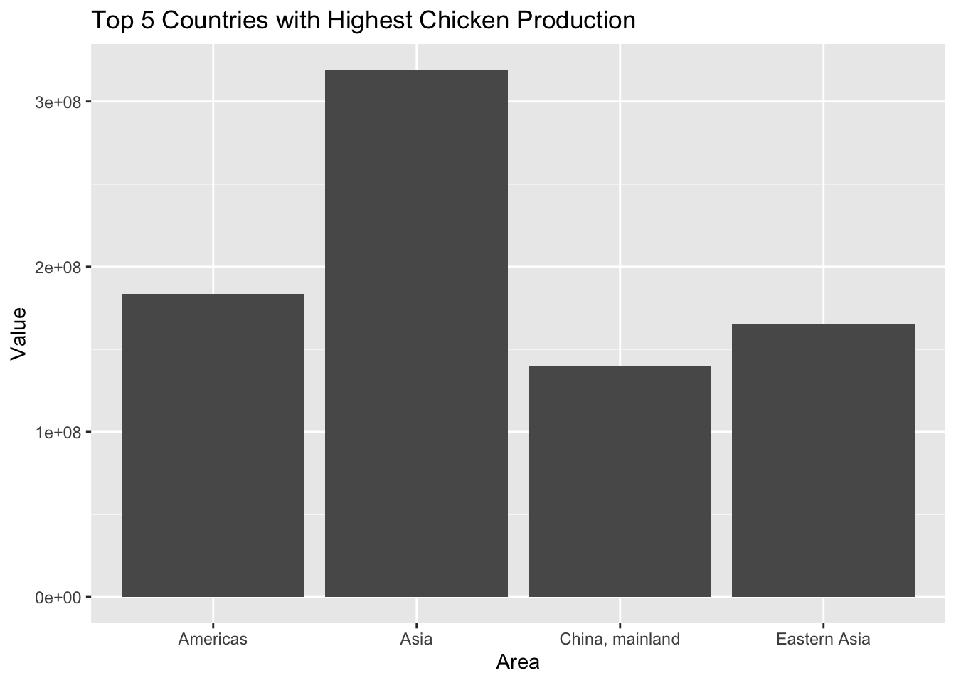

Conclusion

The dataset contains a report for live poultry production for around 248 countries and regions, from the years 1961-2018, with the data gathered by the FAO, showing that chicken is the most produced bird-type and the highest production of chicken is from the Asian region.