library(tidyverse)

knitr::opts_chunk$set(echo = TRUE, warning=FALSE, message=FALSE)DACSS 601 Final Project: Ishan Bhardwaj
final_project
Analysis of Real Estate data
Introduction
One of the most popular fields of investment in the United States is real estate as it can significantly increase one’s net worth and act as a marker of dramatic personal gain. It is approached with tireless research on the most favorable locations, size and composition of the residence, price, and numerous other detailed features. It can be a time-consuming process to look for a suitable match in the real estate world, so being knowledgeable about historical housing trends and important features to look out for can help us avoid loopholes. This leads me to the dataset I am utilizing in this report: an exhaustive table of general physical residence features and historical data, along with listing statuses and prices. In this dataset, each case/row represents a residence and the primary variables one may want to observe.
The research question I wish to answer is: “Which primary variables contribute most to real estate prices and what patterns exist between them?” I hope to find certain variables that show a traditionally greater impact than others on housing prices. I will also be analyzing certain variables’ impact on others because simply knowing the most influential factor may not be enough; an impactful variable may be wholly dependent on the trends observed in other variables.
It is important to investigate this data because if we locate markers that have drastically skewed residence prices, they could carry more weight in prediction-based mechanisms like Machine Learning models. It could make our research on real estate easier because we would know what key variables to consider first and filter our needs around them.
Data
The data I will be analyzing in this report is from the USA Real Estate Dataset on Kaggle, where it is updated every 2-4 weeks. The source of the data in this dataset is realtor.com. Each case/row of this dataset represents a residence in the United States along with its listing status, number of bedrooms and bathrooms, land occupancy measured in acres, location, size, date of previous sale, and price. This dataset contains entries for locations spread all across the US, so we should expect a good amount of diversity in prices.
Reading the data
The first step is to load the dataset into R.
realtor <- read_csv("IshanBhardwaj_FinalProjectData/realtor-data.csv")
realtor <- rename(realtor, "listing_status" = "status", "acre_lot_size" = "acre_lot")
Interpreting the data
We can now obtain dimensional and variable information from this dataset.
dim(realtor)[1] 206000 10colnames(realtor) [1] "listing_status" "bed" "bath" "acre_lot_size"
[5] "city" "state" "zip_code" "house_size"
[9] "prev_sold_date" "price" unique(realtor$listing_status)[1] "for_sale" "ready_to_build"min(realtor$prev_sold_date, na.rm = TRUE)[1] "1901-01-01"max(realtor$prev_sold_date, na.rm = TRUE)[1] "2022-12-01"This dataset contains 206000 rows and 10 columns. The columns/variables, as discussed, are primary variables a potential buyer/investor may observe when performing real estate research. I have renamed some of these variables for clarity. Essentially, each case is identified by a listing status: whether it is “for sale” or “ready to build.” It contains the number of bedrooms and bathrooms of the residence, its location by state, city, and ZIP code, its size in square feet, its land occupancy in acres, its date of last sale and its price in USD. These cases range from sales made in the beginning of 1901 to the end of 2022. The prices either correspond to the current price or the date of last sale if the residence was sold relatively recently. From all this information, it will become seamless to zero in on the actual residence location for in-person inspections.
The cases are presented as a combination of character strings, numeric data, and dates, like so:
head(realtor)This dataset is also “tidy” because each relevant variable has its own column, each case/listing has its own row, and each value has its own cell. There are multiple occurrences of missing data (“NA”) which is inevitable given the range of sale dates for the listings. These will be dealt with when we approach the analysis section of this report. There is also no need to make any mutations or recodings of variable values as all values are in the correct format.
Summary Statistics
The major variables of interest for this report are bed, bath, acre_lot_size, city, state, house_size, prev_sold_date, and price. We can develop some of their summary statistics:
realtor %>%
  select("bed", "bath", "acre_lot_size", "house_size", "price") %>%
  summarize_all(list(mean = mean, median = median, sd = sd), na.rm = TRUE)
On average, the dataset contains listings with ~3.5 bedrooms and ~2.5 bathrooms, with a land occupancy of ~8.5 acres. However, there is lot of variance for each of these values, which means that the distribution of the listings is relatively evenly spread. There must be a non-negligible number of listings at the upper and lower ends of the bedroom, bathroom, and land occupancy spectrum. The centers of these distributions are most likely dealing with houses for families with 3-5 members. We see similar distribution trends for the residence prices, whose mean is ~$870000, which is in the expected range for a family home. These spread-out distributions are expected given the number of cases in this dataset and the range of sale dates. While these statistics confirm that many different types of residences exist in this dataset, the major converging point is most likely 3-5 member family homes.
Data Analysis Plan
I plan to divide the analysis using visualizations into two steps: filtering the original dataset by locating variable values that do not have much effect on price, and using the fully filtered dataset to observe relationships between the variables of interest and residence prices.
The first plot will observe the change in prices over time, and filter out dates that have stagnant prices. The second plot will check the prices of residences in different locations, and filter out locations that contain similar residence costs throughout the dataset. The third plot will check the relationship between land occupancy and house size; if a positive relationship is determined, we can use only one of the two variables in our analyses. The remaining plots will be comparisons of the numerical variables of interest against the price.
Data Filtering
Since we are trying to find the effect of multiple variables on residence prices, let us analyze the prices themselves over time first. A valid variable that records time is prev_sold_date.
ggplot(realtor, aes(x = prev_sold_date, y = price, color = "Price")) +
  geom_line() +
  theme_minimal() +
  labs(title = "Line Plot", subtitle = "Date of last sale vs Price", x = "Date of last sale", y = "Price", color = "Color")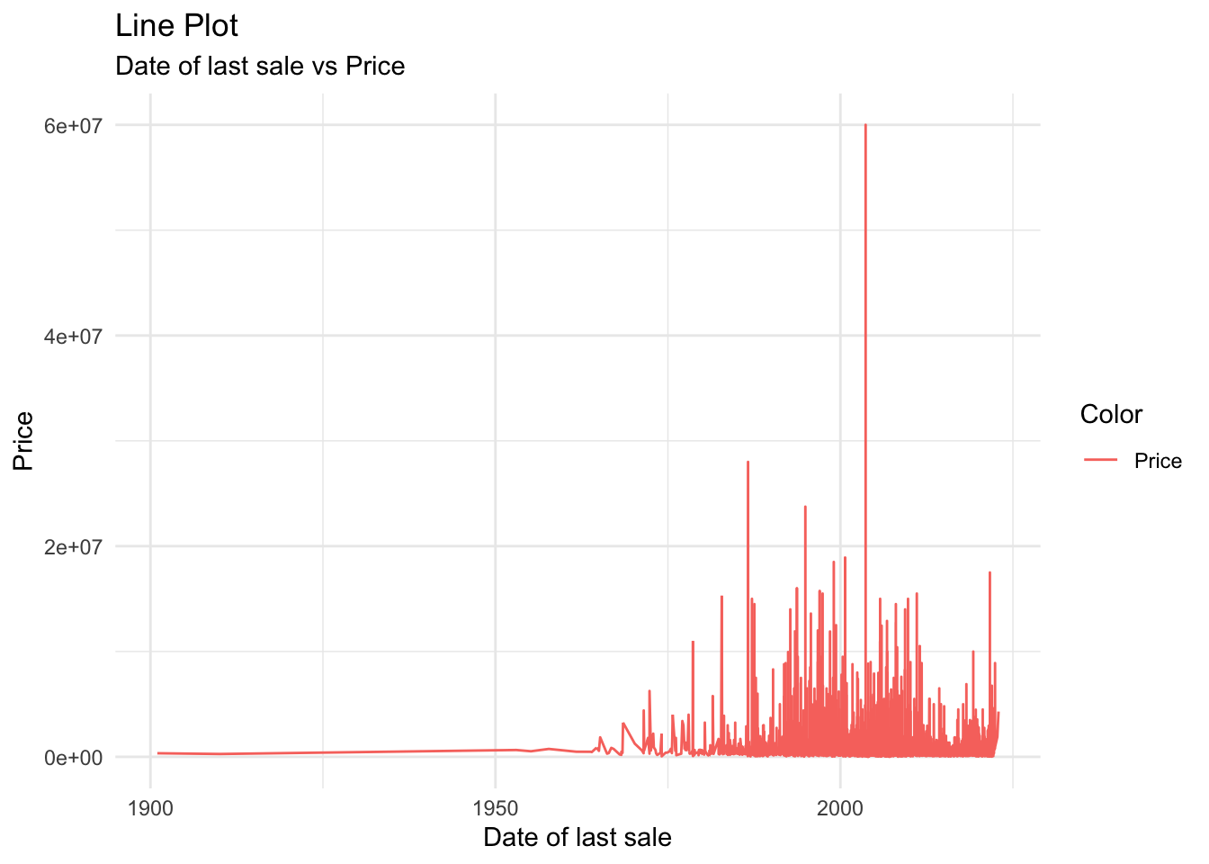
As seen in this graph, residence prices show low variance until ~1975, after which they start dramatically spiking. We can remove the cases with a year of last sale less than 1975 because without much fluctuation in price, we will not be able to tell if one variable had a greater impact than another.
realtor <- filter(realtor, year(prev_sold_date) >= 1975)
realtor
We can also analyze the price distribution depending on the state where the residence is located. This will tell us which areas have a high cost of living and can possibly yield in further filtering of the dataset.
ggplot(realtor, aes(x = state, y = price)) +
  geom_boxplot(outlier.color = "red") +
  theme_minimal() +
  theme(axis.text.x=element_text(angle=90, hjust=1)) +
  labs(title = "Box Plot", subtitle = "State vs Price", x = "State", y = "Price")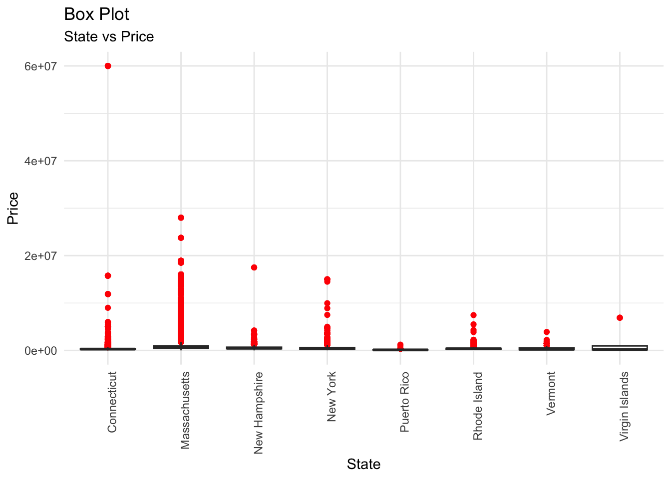
While all the states present in the dataset have similar medians for residence prices, they differ in variance. Massachusetts has the most spread-out outliers followed by Connecticut and New York. The outliers for Puerto Rico and the Virgin Islands are barely spread out, which means that all residences from this dataset for these states present relatively similar prices. This means that we cannot thoroughly observe which variables carry a greater impact on the price for these states. Hence, we can filter out listings located in these states.
copy <- realtor
copy <- filter(copy, state != "Puerto Rico" & state != "Virgin Islands")
copy
We should also find the relation between the land size of the residence and the size of the residence itself. Intuitively, these variables should be proportional to each other, but if we can obtain proof of this relation we will only need to analyze one of these variables’ effects on the price.
ggplot(copy, aes(x = acre_lot_size, y = house_size)) +
  geom_smooth() +
  theme_minimal() +
  labs(title = "Curve Plot", subtitle = "Land Occupancy (acres) vs House Size (sq. ft)", x = "Land Occupancy (acres)", y = "House Size (sq. ft)")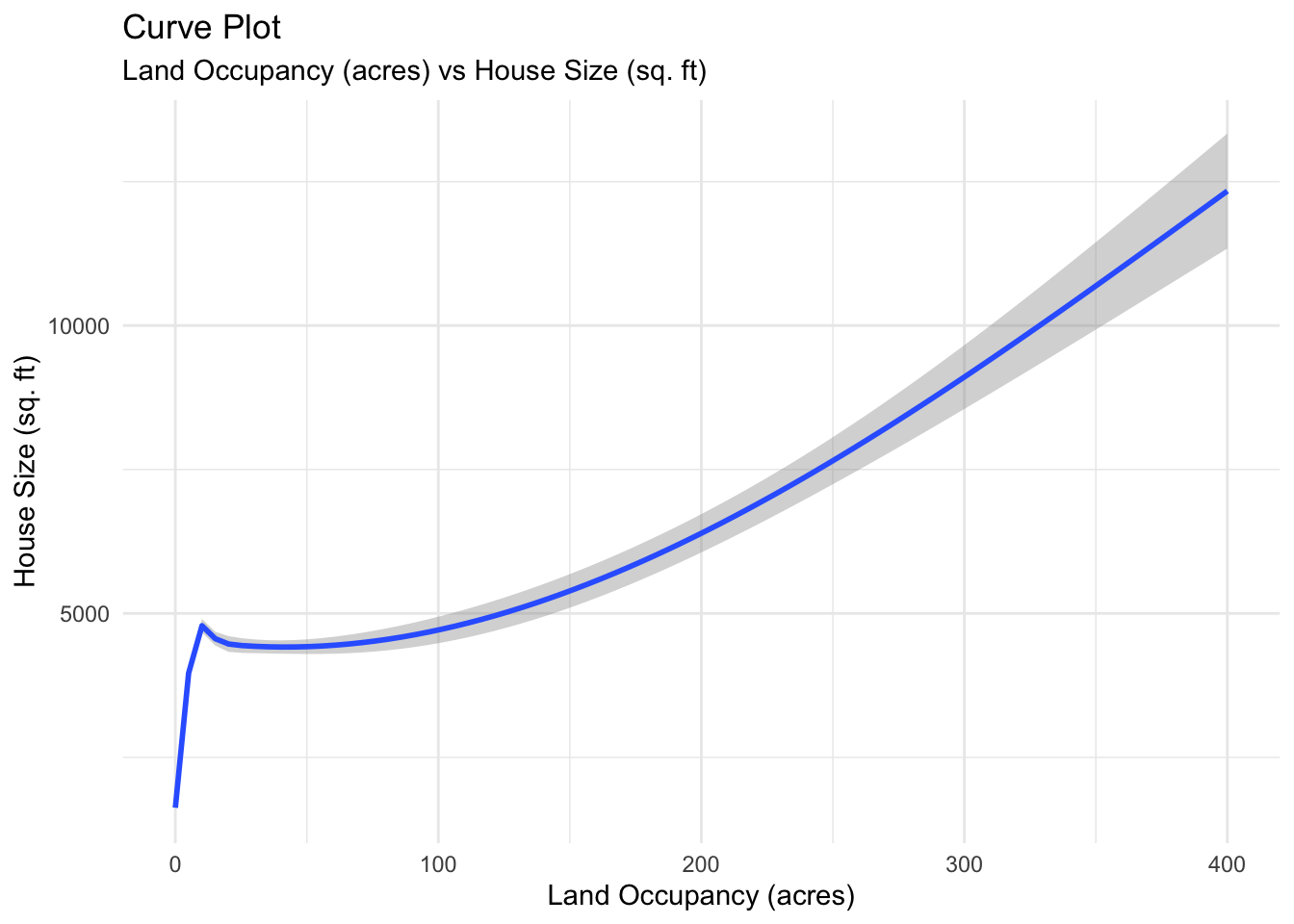
As expected, the general trend is that as the land size increases, the house size increases. Therefore, let us just use the acre_lot_size variable to find out the effect of property size on price.
Visualizations
Now, let us plot the three major numeric variables - bed, bath, and acre_lot_size - against price.
ggplot(copy, aes(x = acre_lot_size, y = price)) +
  geom_point(aes(color = state)) +
  geom_smooth() +
  theme_minimal() +
  labs(title = "Scatterplot", subtitle = "Land Occupancy (acres) vs Price", x = "Land Occupancy (acres)", y = "Price", color = "State")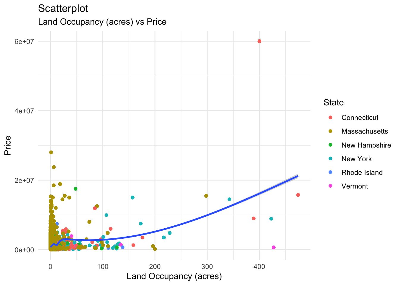
ggplot(copy, aes(x = bed, y = price)) +
  geom_point(aes(color = state)) +
  geom_smooth() +
  theme_minimal() +
  labs(title = "Scatterplot", subtitle = "No. of bedrooms vs Price", x = "No. of bedrooms", y = "Price", color = "State")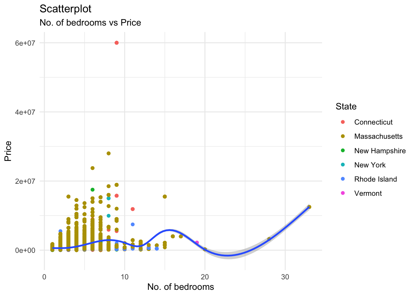
ggplot(copy, aes(x = bath, y = price)) +
  geom_point(aes(color = state)) +
  geom_smooth() +
  theme_minimal() +
  labs(title = "Scatterplot", subtitle = "No. of bathrooms vs Price", x = "No. of bathrooms", y = "Price", color = "State")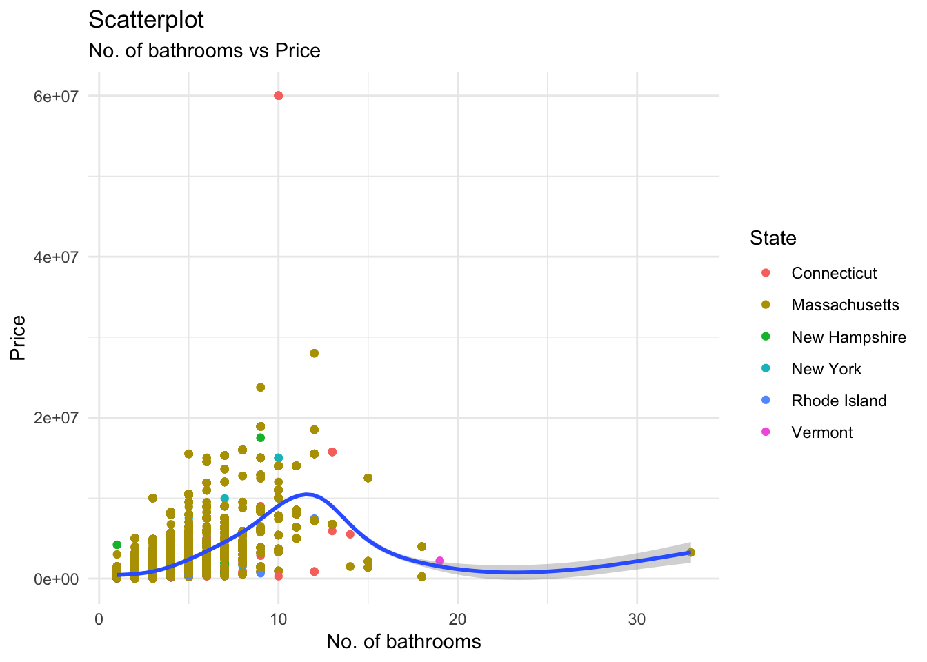
The land occupancy shows us a smooth and gradual increase in price as its size increases. However, the effective upward sloping occurs only after most land occupancy sizes in the dataset have been considered, i.e; between 0-150 acres where most of the land sizes from the dataset lie, the price curve has a relatively horizontal, constant slope. It is only between 200-400 acres that the actual upward slope starts occurring, but there is only a small number of residences having this land size. For the bedrooms plot, we see a somewhat similar trend; in the range 0-10 bedrooms which covers most houses, the slope of the curve remains relatively unaltered. It experiences a sharp increase at the end but this is due to a single data point, which is negligible considering the number of entries in our dataset. Hence, that increase can be ignored on account of “noise”.
However, the bathrooms curve is the only one that shows an increase in price in the range where most of the dataset cases lie. As we can see, a majority of the residences from this dataset have 0-15 bathrooms. It is in this range where the price experiences a notable increase, contrary to the trends in the other variables. Hence, we can conclude that the number of bathrooms has the most effect on the prices in this dataset.
To confirm our findings, let us calculate correlation values for land size vs price, no. of bedrooms vs price, and no. of bathrooms vs price. We must first ensure that we remove missing data entries (“NA”) so the correlations are made based on the existing values.
corr_copy <- copy
corr_copy <- corr_copy %>%
  filter(!is.na(acre_lot_size)) %>%
  filter(!is.na(price))

# Correlation between land size and price
cor(corr_copy$acre_lot_size, corr_copy$price)
[1] 0.298269corr_copy <- copy
corr_copy <- corr_copy %>%
filter(!is.na(bed)) %>%
filter(!is.na(price))
# Correlation between number of bedrooms and price
cor(corr_copy$bed, corr_copy$price)[1] 0.3185935corr_copy <- copy
corr_copy <- corr_copy %>%
filter(!is.na(bath)) %>%
filter(!is.na(price))
# Correlation between number of bathrooms and price
cor(corr_copy$bath, corr_copy$price)[1] 0.6087761As expected, the number of bathrooms shows the maximum correlation to the price of a residence out of the these numerical variables.
Conclusion
This report was made to analyze the effects of different variables of primary consideration on the prices of residences in a large dataset of real estate cases in the United States across many years, and its primary objective was to locate the variables that had the most effect on residence prices. From the analyses I have performed, I can conclude that for locations ranging in those present in the dataset, the location that has the strongest effect on prices is Massachusetts due to its relatively large outlier spread in the boxplot of state vs price. The numerical variable that has the strongest effect on price is the number of bathrooms present in the residence, and this was found out through visualizations and confirmed by correlation tests.
While this analysis is thorough, I believe that it could be scaled up because I found that the number of states present in the dataset were quite few. I believe that with the inclusion of more high cost-of-living states like California, the results of this report could change. I believe that this could help in future prospects for the research conducted here, such as grouping different states by their variables that have the most effect on price and locating relationships between these variables.
Bibliography
R Core Team. (2021). R: A language and environment for statistical computing. R Foundation for Statistical Computing, Vienna, Austria. URL: https://www.R-project.org/
Sakib, A. S. (2023). USA Real Estate Dataset. Retrieved May 22, 2022, from Kaggle: https://www.kaggle.com/datasets/ahmedshahriarsakib/usa-real-estate-dataset?resource=download