library(tidyverse)
library(ggplot2)
library(readxl)

knitr::opts_chunk$set(echo = TRUE, warning=FALSE, message=FALSE)Challenge 5 - StateCounty Visualizations
state_county
Joseph Vincent
challenge_5
Introduction to Visualization
Reading in StateCounty data
- StateCounty2012.xls ⭐⭐⭐
#reading in StateCounty data
#skipping first 2 blank rows
#Selecting columns with data
#Filtering out aggregate rows
#Filtering out row with note about no addresx
StateCounty <- read_xls("_data/StateCounty2012.xls",
                        skip = 2)
StateCounty <- StateCounty %>%
  select(STATE, COUNTY, TOTAL) %>%
  filter(!str_detect(STATE, "address"))

head(StateCounty)
# A tibble: 6 × 3
STATE COUNTY TOTAL
<chr> <chr> <dbl>
1 AE APO 2
2 AE Total1 <NA> 2
3 AK ANCHORAGE 7
4 AK FAIRBANKS NORTH STAR 2
5 AK JUNEAU 3
6 AK MATANUSKA-SUSITNA 2#recoding the military designation observation
StateCounty[2986, 1] = "MILITARY"
StateCounty[2986, 3] = 1
tail(StateCounty)# A tibble: 6 × 3
STATE COUNTY TOTAL
<chr> <chr> <dbl>
1 WY WASHAKIE 10
2 WY WESTON 37
3 WY Total <NA> 2876
4 Grand Total <NA> 255432
5 CANADA <NA> 662
6 MILITARY <NA> 1#finding the number of counties excluding aggregates
StateCounty %>%
filter(!str_detect(STATE, "Total")) %>%
dim_desc()[1] "[2,932 x 3]"#finding the mean and median by state
StateCounty %>%
filter(str_detect(STATE, "Total")) %>%
summarize(Mean = mean(TOTAL, na.rm = TRUE),
Median = median(TOTAL, na.rm = TRUE),
Max = max(TOTAL, na.rm = TRUE),
Min = min(TOTAL, na.rm = TRUE))# A tibble: 1 × 4
Mean Median Max Min
<dbl> <dbl> <dbl> <dbl>
1 9460. 3514. 255432 1#finding the mean and median by county
StateCounty %>%
filter(!str_detect(STATE, "Total")) %>%
summarize(Mean = mean(TOTAL, na.rm = TRUE),
Median = median(TOTAL, na.rm = TRUE),
Max = max(TOTAL, na.rm = TRUE),
Min = min(TOTAL, na.rm = TRUE))# A tibble: 1 × 4
Mean Median Max Min
<dbl> <dbl> <dbl> <dbl>
1 87.3 21 8207 1Briefly describe the data
The StateCounty dataset is describing the number of employees for a specific organization in each county of the United States. There are also aggregate values for number of employees in each state. There are is also data on the number of employees in Canada and on military bases abroad.
There are a total of 2,932 counties with employees. They are spread across all US states.
The largest state has over 250,000 emoployees, with the state mean being around 9,000 and the state median being around 3,500.
The largest individual county has over 8,000 employees, with the county mean being around 90 employees and the county median being about 20.
Tidy Data (as needed)
The data is already tidy, but as you can see the aggregate state totals will need to be accounted for when the data is analyzed and visualized.
The single military base employee was missing data, and this has been corrected.
unique(StateCounty$STATE) [1] "AE" "AE Total1" "AK" "AK Total" "AL"
[6] "AL Total" "AP" "AP Total1" "AR" "AR Total"
[11] "AZ" "AZ Total" "CA" "CA Total" "CO"
[16] "CO Total" "CT" "CT Total" "DC" "DC Total"
[21] "DE" "DE Total" "FL" "FL Total" "GA"
[26] "GA Total" "HI" "HI Total" "IA" "IA Total"
[31] "ID" "ID Total" "IL" "IL Total" "IN"
[36] "IN Total" "KS" "KS Total" "KY" "KY Total"
[41] "LA" "LA Total" "MA" "MA Total" "MD"
[46] "MD Total" "ME" "ME Total" "MI" "MI Total"
[51] "MN" "MN Total" "MO" "MO Total" "MS"
[56] "MS Total" "MT" "MT Total" "NC" "NC Total"
[61] "ND" "ND Total" "NE" "NE Total" "NH"
[66] "NH Total" "NJ" "NJ Total" "NM" "NM Total"
[71] "NV" "NV Total" "NY" "NY Total" "OH"
[76] "OH Total" "OK" "OK Total" "OR" "OR Total"
[81] "PA" "PA Total" "RI" "RI Total" "SC"
[86] "SC Total" "SD" "SD Total" "TN" "TN Total"
[91] "TX" "TX Total" "UT" "UT Total" "VA"
[96] "VA Total" "VT" "VT Total" "WA" "WA Total"
[101] "WI" "WI Total" "WV" "WV Total" "WY"
[106] "WY Total" "Grand Total" "CANADA" "MILITARY" Before creating some visualizations of the data, it will be easier to create two data sets that include the county totals and state totals respectively.
#creating a dataset without aggregates for ease of plotting
StateCountyNoAggregates <- StateCounty %>%
  filter(!str_detect(STATE, "Total"))

unique(StateCountyNoAggregates$STATE)
[1] "AE" "AK" "AL" "AP" "AR" "AZ"
[7] "CA" "CO" "CT" "DC" "DE" "FL"
[13] "GA" "HI" "IA" "ID" "IL" "IN"
[19] "KS" "KY" "LA" "MA" "MD" "ME"
[25] "MI" "MN" "MO" "MS" "MT" "NC"
[31] "ND" "NE" "NH" "NJ" "NM" "NV"
[37] "NY" "OH" "OK" "OR" "PA" "RI"
[43] "SC" "SD" "TN" "TX" "UT" "VA"
[49] "VT" "WA" "WI" "WV" "WY" "CANADA"
[55] "MILITARY"#creating a dataset with only the state aggregates for ease of plotting
StateCountyAggregates <- StateCounty %>%
filter(str_detect(STATE, "Total")) %>%
filter(!str_detect(STATE, "Grand Total")) %>%
select(STATE, TOTAL) %>%
separate(STATE, into = c("STATE", "delete"), sep = " ") %>%
select(STATE, TOTAL)
head(StateCountyAggregates)# A tibble: 6 × 2
STATE TOTAL
<chr> <dbl>
1 AE 2
2 AK 103
3 AL 4257
4 AP 1
5 AR 3871
6 AZ 3153Univariate Visualizations
Below you can see a few different distributions: The first is a plot of the distribution of county employee totals, for those containing less than 500 employees. This was done as there are some extreme outliers in the data set that would make it harder to visualize.
As you can see, the vast majority of counties have a small number of employees.
In the second plot, you can see the distribution of state employee totals. Most states have around 5,000 or fewer employees, but there are some outliers which will be further described in later plots.
#Plotting the distribution of county employee totals
StateCountyNoAggregates %>%
  filter(TOTAL < 500) %>%
  ggplot(aes(TOTAL)) +
    geom_histogram(binwidth=3, fill="#b3697a", alpha=0.9) +
    ggtitle("Distribution of County Employees (Fewer than 500)")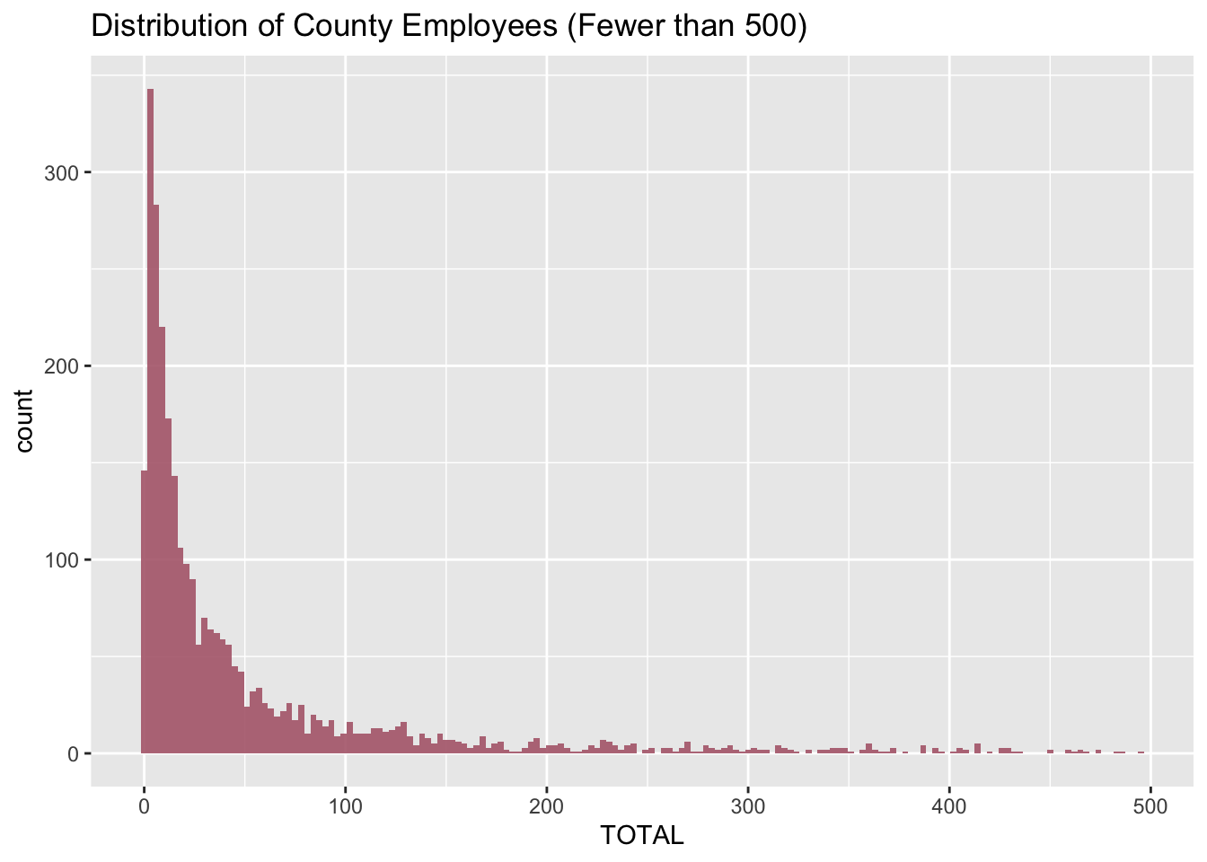
#plotting the distribution of state employee totals
ggplot(StateCountyAggregates, aes(TOTAL)) +
  geom_histogram(fill="#69b3a2", alpha = 0.9) +
  ggtitle("Distribution of State Employees")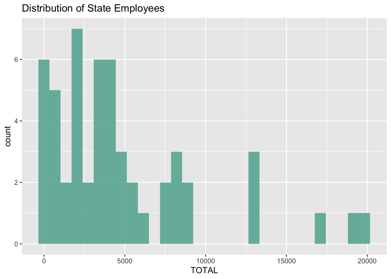
Bivariate Visualization(s)
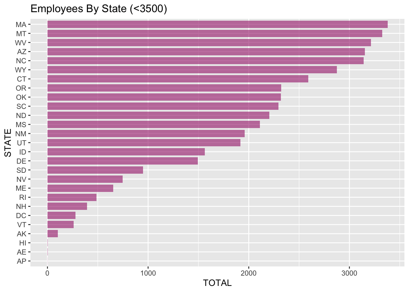
Next we will take a look at a detailed breakdown of employees by state. The two bar-plots below make it easy to visualize the number of employees in each state and their order. I split this into two charts, one above the mean and one below the mean, simply to declutter the plots and make them easier to read.
#plotting distribution of employees by state for those with over 2000 employees
#using fct_reorder to order from greatest to least
StateCountyAggregates %>%
  filter(TOTAL >= 3500) %>%
  mutate(STATE = fct_reorder(STATE, TOTAL)) %>%
  ggplot(aes(x=STATE, y=TOTAL)) +
  geom_bar(stat = "identity", fill="#f68060", alpha=.6, width=.8) +
  coord_flip() +
  ggtitle("Employees By State (>=3500)")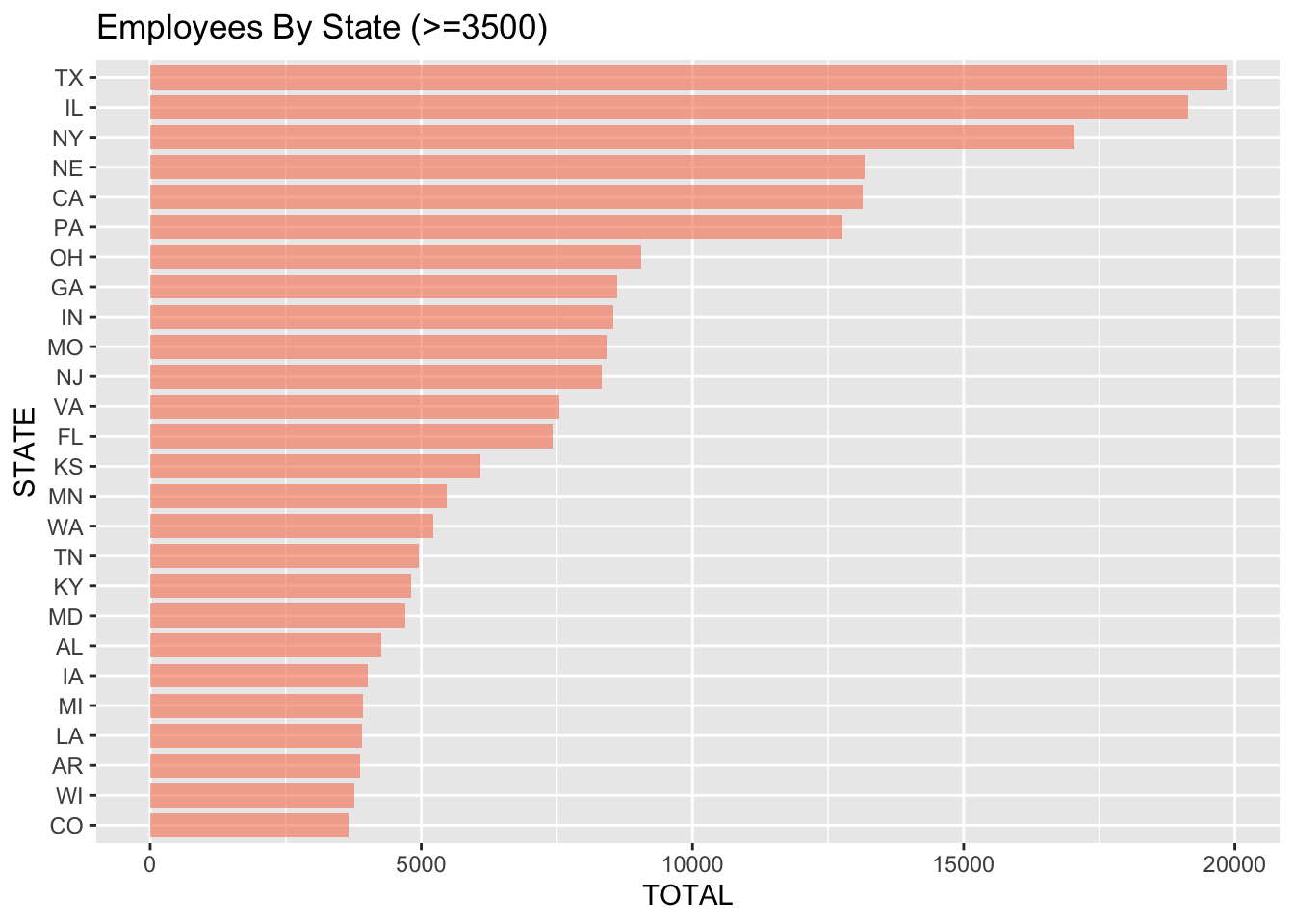
#plotting distribution of employees by state for those with less than 2000 employees
#using fct_reorder to order from greatest to least
StateCountyAggregates %>%
  filter(TOTAL < 3500) %>%
  mutate(STATE = fct_reorder(STATE, TOTAL)) %>%
  ggplot(aes(x=STATE, y=TOTAL)) +
  geom_bar(stat = "identity", fill="#a42678", alpha=.6, width=.8) +
  coord_flip() +
  ggtitle("Employees By State (<3500)")