library(tidyverse)
library(ggplot2)
library(lubridate)

knitr::opts_chunk$set(echo = TRUE, warning=FALSE, message=FALSE)Challenge 7 - Hotel Bookings
challenge_7
hotel_bookings
JosephVincent
Visualizing Multiple Dimensions
Read in data (hotel bookings)
- hotel_bookings ⭐⭐⭐
hoteldata <- read.csv("_data/hotel_bookings.csv")
head(hoteldata)
hotel is_canceled lead_time arrival_date_year arrival_date_month
1 Resort Hotel 0 342 2015 July
2 Resort Hotel 0 737 2015 July
3 Resort Hotel 0 7 2015 July
4 Resort Hotel 0 13 2015 July
5 Resort Hotel 0 14 2015 July
6 Resort Hotel 0 14 2015 July
arrival_date_week_number arrival_date_day_of_month stays_in_weekend_nights
1 27 1 0
2 27 1 0
3 27 1 0
4 27 1 0
5 27 1 0
6 27 1 0
stays_in_week_nights adults children babies meal country market_segment
1 0 2 0 0 BB PRT Direct
2 0 2 0 0 BB PRT Direct
3 1 1 0 0 BB GBR Direct
4 1 1 0 0 BB GBR Corporate
5 2 2 0 0 BB GBR Online TA
6 2 2 0 0 BB GBR Online TA
distribution_channel is_repeated_guest previous_cancellations
1 Direct 0 0
2 Direct 0 0
3 Direct 0 0
4 Corporate 0 0
5 TA/TO 0 0
6 TA/TO 0 0
previous_bookings_not_canceled reserved_room_type assigned_room_type
1 0 C C
2 0 C C
3 0 A C
4 0 A A
5 0 A A
6 0 A A
booking_changes deposit_type agent company days_in_waiting_list customer_type
1 3 No Deposit NULL NULL 0 Transient
2 4 No Deposit NULL NULL 0 Transient
3 0 No Deposit NULL NULL 0 Transient
4 0 No Deposit 304 NULL 0 Transient
5 0 No Deposit 240 NULL 0 Transient
6 0 No Deposit 240 NULL 0 Transient
adr required_car_parking_spaces total_of_special_requests reservation_status
1 0 0 0 Check-Out
2 0 0 0 Check-Out
3 75 0 0 Check-Out
4 75 0 0 Check-Out
5 98 0 1 Check-Out
6 98 0 1 Check-Out
reservation_status_date
1 2015-07-01
2 2015-07-01
3 2015-07-02
4 2015-07-02
5 2015-07-03
6 2015-07-03dim(hoteldata)[1] 119390 32Briefly describe the data
The data set consists of information about hotel stays between July 2015 and August 2017. There are 33 variables and over 100,000 stays.
Some of the key variables worth mentioning are:
Type of hotel (either Resort Hotel or City Hotel) - presumably this is data from a booking service that has multiple hotel customers
Arrival date, which is broken into several columns including year, month, day, week, etc.
Occupants of each stay (adults, children, babies)
Market segments and distribution channels
Average daily rate (ADR) - from some research this seems to be the average rate across all rooms for a given date
Lead time - or the time from booking to arrival
Tidy Data (as needed) and Mutating
One of the main problems with the data set for analysis purposes is that the arrival date is broken into various character columns. To fix this, I mutated the the arrival month names into numeric values, and then used lubridate to create a new single column for arrival date in the proper format.
Some of the variables (such as whether the stay was canceled, or whether it was a repeat guest) were in binary (0,1) format. I converted these into logical TRUE/FALSE variables.
I also created a new column for total nights stayed, which combined week and weekend nights stayed.
After completing these steps I would expect to see: 33(original) - 4 (individual arrival date columns) + 1 (new arrival date) + 1 (custom arrival date with month only for further anlysis) = 31 columns Which is confirmed by my sanity check below.
You can also see that the new “arrival_date” column is in date format.
#converting months to numerics to use in make date
hoteldatatidy <- hoteldata %>%
  mutate(monthnumeric = case_when(
    `arrival_date_month` == "January" ~ 1,
    `arrival_date_month` == "February" ~ 2,
    `arrival_date_month` == "March" ~ 3,
    `arrival_date_month` == "April" ~ 4,
    `arrival_date_month` == "May" ~ 5,
    `arrival_date_month` == "June" ~ 6,
    `arrival_date_month` == "July" ~ 7,
    `arrival_date_month` == "August" ~ 8,
    `arrival_date_month` == "September" ~ 9,
    `arrival_date_month` == "October" ~ 10,
    `arrival_date_month` == "November" ~ 11,
    `arrival_date_month` == "December" ~ 12)) %>%

  #turning separate arrival date columns into a single arrival date
  mutate(arrival_date = make_date(year = arrival_date_year, month = monthnumeric, day = arrival_date_day_of_month)) %>%

  #making custom month-only column
  mutate(arrival_month = make_date(year = arrival_date_year, month = monthnumeric)) %>%

  #mutating binary 0/1 columns to be TRUE/FALSE
  mutate(is_canceled = case_when(
    `is_canceled` == 0 ~ FALSE,
    `is_canceled` == 1 ~ TRUE,)) %>%
  mutate(is_repeated_guest = case_when(
    `is_repeated_guest` == 0 ~ FALSE,
    `is_repeated_guest` == 1 ~ TRUE,)) %>%

  #combining week and weekend nights stayed for a total column
  mutate(total_nights_stayed = stays_in_weekend_nights + stays_in_week_nights) %>%

  #deselecting unused columns
  select(-c(`monthnumeric`, `arrival_date_day_of_month`, `arrival_date_week_number`, `arrival_date_month`, `arrival_date_year`))

#doing some sanity checks
head(hoteldatatidy$arrival_date)
[1] "2015-07-01" "2015-07-01" "2015-07-01" "2015-07-01" "2015-07-01"
[6] "2015-07-01"dim(hoteldatatidy)[1] 119390 31##Preparing data for visualization
Before creating a time series visualization, I wanted to create a summary table, showing the means of key values like Lead Time, ADR and Total Nights Stayed, grouped by hotel type.
monthlymeansbyhoteltype <- hoteldatatidy %>%
  group_by(arrival_month, hotel) %>%
  summarize(mean_lead_time = mean(lead_time),
            mean_adr = mean(adr),
            mean_stay = mean(total_nights_stayed))
head(monthlymeansbyhoteltype)
# A tibble: 6 × 5
# Groups: arrival_month [3]
arrival_month hotel mean_lead_time mean_adr mean_stay
<date> <chr> <dbl> <dbl> <dbl>
1 2015-07-01 City Hotel 181. 69.8 2.69
2 2015-07-01 Resort Hotel 70.5 126. 5.06
3 2015-08-01 City Hotel 114. 77.7 2.72
4 2015-08-01 Resort Hotel 74.3 156. 5.43
5 2015-09-01 City Hotel 114. 101. 2.73
6 2015-09-01 Resort Hotel 144. 80.9 5.13Visualization with Multiple Dimensions
As we saw in the previous challenge, mean Lead Time and ADR tracked each other closely, tending to rise in the busier summer months and fall in the winter months.
To expand upon this, I’d like to add the additional dimensions of hotel type (city vs resort) and mean length of stay to see if they follow the similar trends.
Mean lead time by month and hotel type
Using our means table, below I have plotted a time-series chart of mean lead time, with each line representing a hotel type. They trend similarly over time, though the lead times for the resort hotel appear to be slightly more extreme in either direction. Particularly in the winter months, lead time for the resort hotel is quite low. This makes sense, as you’d expect that people might not plan far in advance for a resort trip in the winter.
#creating a ggplot using monthlymeans table
#setting the x axis as arrival date
leadtimebyhotel <- ggplot(monthlymeansbyhoteltype, aes(x = arrival_month, y = mean_lead_time, color = hotel)) +

  geom_line() +

  #setting y scale and creating an additional y axis on the right side
  scale_y_continuous(name = "Mean Lead Time (Days)") +
  scale_x_date(date_labels = "%b %y", date_breaks = "2 months", name = "Month") +

  #setting theme options
  theme_minimal() +
  theme(axis.text.x=element_text(angle=60, hjust=1)) +
  ggtitle("Mean Lead Time by Month and Hotel")

#plotting
leadtimebyhotel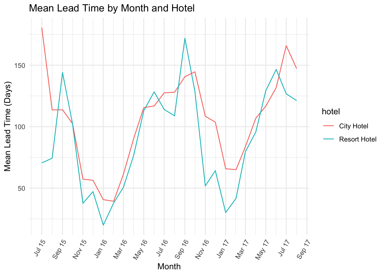
Mean lead time by month and hotel type, scaled by stay length
To take this a step further, I will look at whether stay length is also greater during months when lead time is.
Below I’ve graphed the same data as before, but this time used points to represent each monthly mean. Triangles represent the resort hotel, while circles represent the city hotel.
As you can see from the stay length scale (and color gradient) the mean resort hotel stays tend to be longer than the city hotel stays. The hotel stays in general seem to be longer during the summer months, but this is much clearer for the resort stays.
leadtimeandstay <- ggplot(monthlymeansbyhoteltype, aes(x = arrival_month, y = mean_lead_time, size = mean_stay, color = mean_stay, shape = hotel)) +

  geom_point() +

    #setting y scale and creating an additional y axis on the right side
  scale_y_continuous(name = "Mean Lead Time (Days)") +
  scale_x_date(date_labels = "%b %y", date_breaks = "2 months", name = "Month") +

  #setting theme options
  theme_minimal() +
  theme(axis.text.x=element_text(angle=60, hjust=1)) +
  ggtitle("Mean Lead Time by Month (Scaled by Length of Stay)") +
  guides(color = FALSE) +
  labs(size = "Mean Length of Stay")

leadtimeandstay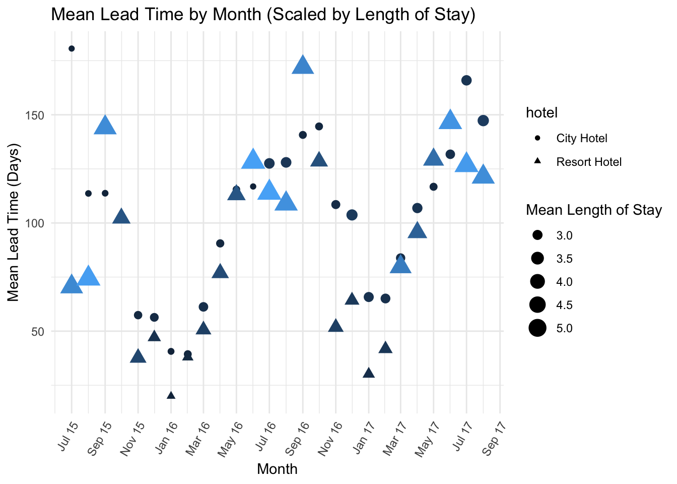
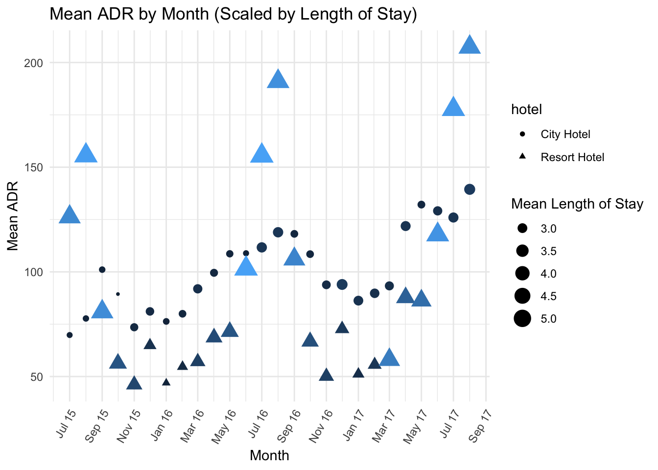
Mean ADR by month and hotel type, scaled by stay length
Finally, I’ll look at the same graph but by ADR instead of lead time.
This results in some interesting findings. The Mean ADR varies much more in for the resort hotel than the city hotel, with the summer “peaks” and winter “valleys” being very pronounced vs the relatively smoother shape of the city hotel ADR plot.
Length of stay is still clearly greater during the summer months for the resort hotel, while length of stay remains relatively consistent throughout the year for the city hotel.
adrandstay <- ggplot(monthlymeansbyhoteltype, aes(x = arrival_month, y = mean_adr, size = mean_stay, color = mean_stay, shape = hotel)) +

  geom_point() +

    #setting y scale and creating an additional y axis on the right side
  scale_y_continuous(name = "Mean ADR") +
  scale_x_date(date_labels = "%b %y", date_breaks = "2 months", name = "Month") +

  #setting theme options
  theme_minimal() +
  theme(axis.text.x=element_text(angle=60, hjust=1)) +
  ggtitle("Mean ADR by Month (Scaled by Length of Stay)") +
  guides(color = FALSE) +
  labs(size = "Mean Length of Stay")

adrandstay