Keith Martin Challenge 3

challenge_3

eggs

Tidy Data: Pivoting

Author

Keith Martin

Published

March 17, 2023

Code

library(tidyverse)
library(googlesheets4)
library(readxl)


knitr::opts_chunk$set(echo = TRUE, warning=FALSE, message=FALSE)

Challenge Overview

In this challenge, I decided to use the excel version of the Organice Poultry Data. Before I could read into the data, I needed to include libraries that allowed me to read in excel files.

Read in data

After reading in the data, I noticed that there we’re three different tabs within the excel file. I decided to use only the data tab as this was the first excel file I have read into R.

Code

### Loading in the libraries of the excel files
excel_sheets("_data/organiceggpoultry.xls")

[1] "Data"                            "Organic egg prices, 2004-13"    
[3] "Organic poultry prices, 2004-13"

I decided to re-name the names of the columns so they we’re more easily identified. This will become helpful later when I pivot the data longer. Additionally, there is a row that needed to be removed from the data that split the egg prices and the chicken prices. By re-naming the cells it is easier to analyze the data.

Code

raw_poulty<-read_excel("_data/organiceggpoultry.xls", 
                         sheet = "Data",
                          range =cell_limits(c(6,2),c(NA,12)),
                          col_names = c("date", "XL_Dozen", "XL_1/2_Doz.", "L_Dozen", "L_1/2_Doz", "Remove", "Ckn_Whole", "Ckn_BS_Breast", "Ckn_Bone_Breast", "Ckn_Whole_legs", "Ckn_Thighs"),
                      
                                        
                        )
raw_poulty %>%
  select(-c(Remove))

# A tibble: 120 × 10
   date  XL_Do…¹ XL_1/…² L_Dozen L_1/2…³ Ckn_W…⁴ Ckn_B…⁵ Ckn_B…⁶ Ckn_W…⁷ Ckn_T…⁸
   <chr>   <dbl>   <dbl>   <dbl>   <dbl>   <dbl>   <dbl> <chr>     <dbl> <chr>  
 1 Jan …    230     132     230     126     198.    646. too few    194. too few
 2 Febr…    230     134.    226.    128.    198.    642. too few    194. 203    
 3 March    230     137     225     131     209     642. too few    194. 203    
 4 April    234.    137     225     131     212     642. too few    194. 203    
 5 May      236     137     225     131     214.    642. too few    194. 203    
 6 June     241     137     231.    134.    216.    641  too few    202. 200.375
 7 July     241     137     234.    134.    217     642. 390.5      204. 199.5  
 8 Augu…    241     137     234.    134.    217     642. 390.5      204. 199.5  
 9 Sept…    241     136.    234.    130.    217     642. 390.5      204. 199.5  
10 Octo…    241     136.    234.    128.    217     642. 390.5      204. 199.5  
# … with 110 more rows, and abbreviated variable names ¹XL_Dozen,
#   ²`XL_1/2_Doz.`, ³`L_1/2_Doz`, ⁴Ckn_Whole, ⁵Ckn_BS_Breast, ⁶Ckn_Bone_Breast,
#   ⁷Ckn_Whole_legs, ⁸Ckn_Thighs

Code

### Display the months for cleaning purposes
raw_poulty %>%
  count(date)

# A tibble: 22 × 2
   date            n
   <chr>       <int>
 1 April          10
 2 August         10
 3 December       10
 4 February        8
 5 February /1     2
 6 Jan 2004        1
 7 Jan 2005        1
 8 Jan 2006        1
 9 Jan 2007        1
10 Jan 2008        1
# … with 12 more rows

Code

### remove that /1 from the February date
raw_poulty_clean <-raw_poulty %>% 
  mutate(date = str_remove(date, " /1"))
### Separate the month and the year, fill the years in for the rest of the months
raw_poulty_clean<-raw_poulty_clean %>%
  separate(date, into=c("month", "year"), sep =" ")%>%
  fill(year)
raw_poulty_clean

# A tibble: 120 × 12
   month    year  XL_Do…¹ XL_1/…² L_Dozen L_1/2…³ Remove Ckn_W…⁴ Ckn_B…⁵ Ckn_B…⁶
   <chr>    <chr>   <dbl>   <dbl>   <dbl>   <dbl> <lgl>    <dbl>   <dbl> <chr>  
 1 Jan      2004     230     132     230     126  NA        198.    646. too few
 2 February 2004     230     134.    226.    128. NA        198.    642. too few
 3 March    2004     230     137     225     131  NA        209     642. too few
 4 April    2004     234.    137     225     131  NA        212     642. too few
 5 May      2004     236     137     225     131  NA        214.    642. too few
 6 June     2004     241     137     231.    134. NA        216.    641  too few
 7 July     2004     241     137     234.    134. NA        217     642. 390.5  
 8 August   2004     241     137     234.    134. NA        217     642. 390.5  
 9 Septemb… 2004     241     136.    234.    130. NA        217     642. 390.5  
10 October  2004     241     136.    234.    128. NA        217     642. 390.5  
# … with 110 more rows, 2 more variables: Ckn_Whole_legs <dbl>,
#   Ckn_Thighs <chr>, and abbreviated variable names ¹XL_Dozen, ²`XL_1/2_Doz.`,
#   ³`L_1/2_Doz`, ⁴Ckn_Whole, ⁵Ckn_BS_Breast, ⁶Ckn_Bone_Breast

This data did not include the year for each month entry. There was also a mistake in the data that needed to be removed.

Additionally, the Chicken Bone Breast and the Chicken Thighs data containted characters rather than numbers. First, I had to change those words to 0. Then, I had to change them to a numerical number, rather than just a character.

Code

ckn_edited<- raw_poulty_clean %>%
  mutate(Ckn_Bone_Breast = recode(Ckn_Bone_Breast, `too few` = "0"),
      Ckn_Thighs = recode(Ckn_Thighs, `too few`="0"))
ckn_edited

# A tibble: 120 × 12
   month    year  XL_Do…¹ XL_1/…² L_Dozen L_1/2…³ Remove Ckn_W…⁴ Ckn_B…⁵ Ckn_B…⁶
   <chr>    <chr>   <dbl>   <dbl>   <dbl>   <dbl> <lgl>    <dbl>   <dbl> <chr>  
 1 Jan      2004     230     132     230     126  NA        198.    646. 0      
 2 February 2004     230     134.    226.    128. NA        198.    642. 0      
 3 March    2004     230     137     225     131  NA        209     642. 0      
 4 April    2004     234.    137     225     131  NA        212     642. 0      
 5 May      2004     236     137     225     131  NA        214.    642. 0      
 6 June     2004     241     137     231.    134. NA        216.    641  0      
 7 July     2004     241     137     234.    134. NA        217     642. 390.5  
 8 August   2004     241     137     234.    134. NA        217     642. 390.5  
 9 Septemb… 2004     241     136.    234.    130. NA        217     642. 390.5  
10 October  2004     241     136.    234.    128. NA        217     642. 390.5  
# … with 110 more rows, 2 more variables: Ckn_Whole_legs <dbl>,
#   Ckn_Thighs <chr>, and abbreviated variable names ¹XL_Dozen, ²`XL_1/2_Doz.`,
#   ³`L_1/2_Doz`, ⁴Ckn_Whole, ⁵Ckn_BS_Breast, ⁶Ckn_Bone_Breast

Code

ckn_edited$Ckn_Bone_Breast<-as.numeric(ckn_edited$Ckn_Bone_Breast)
ckn_edited$Ckn_Thighs<-as.numeric(ckn_edited$Ckn_Thighs)
ckn_edited

# A tibble: 120 × 12
   month    year  XL_Do…¹ XL_1/…² L_Dozen L_1/2…³ Remove Ckn_W…⁴ Ckn_B…⁵ Ckn_B…⁶
   <chr>    <chr>   <dbl>   <dbl>   <dbl>   <dbl> <lgl>    <dbl>   <dbl>   <dbl>
 1 Jan      2004     230     132     230     126  NA        198.    646.      0 
 2 February 2004     230     134.    226.    128. NA        198.    642.      0 
 3 March    2004     230     137     225     131  NA        209     642.      0 
 4 April    2004     234.    137     225     131  NA        212     642.      0 
 5 May      2004     236     137     225     131  NA        214.    642.      0 
 6 June     2004     241     137     231.    134. NA        216.    641       0 
 7 July     2004     241     137     234.    134. NA        217     642.    390.
 8 August   2004     241     137     234.    134. NA        217     642.    390.
 9 Septemb… 2004     241     136.    234.    130. NA        217     642.    390.
10 October  2004     241     136.    234.    128. NA        217     642.    390.
# … with 110 more rows, 2 more variables: Ckn_Whole_legs <dbl>,
#   Ckn_Thighs <dbl>, and abbreviated variable names ¹XL_Dozen, ²`XL_1/2_Doz.`,
#   ³`L_1/2_Doz`, ⁴Ckn_Whole, ⁵Ckn_BS_Breast, ⁶Ckn_Bone_Breast

The original clean data had 12 columns and 120 rows.

Code

ncol(ckn_edited)

[1] 12

Code

nrow(ckn_edited)

[1] 120

Briefly describe the data

I pivoted the data to make the type of item (egg, or chicken meat) show in one column rather than have each one in their own columns. This makes it much easier to analyse the summary statistics.

Code

###pivot the data to longer version for eggs data set
eggs_longer<- pivot_longer(ckn_edited,  cols=c("XL_Dozen", "XL_1/2_Doz.", "L_Dozen", "L_1/2_Doz", "Ckn_Whole", "Ckn_BS_Breast", "Ckn_Bone_Breast", "Ckn_Whole_legs", "Ckn_Thighs"), 
               names_to = "eggType/cknType",
               values_to = "avgPrice"
  )
eggs_longer

# A tibble: 1,080 × 5
   month    year  Remove `eggType/cknType` avgPrice
   <chr>    <chr> <lgl>  <chr>                <dbl>
 1 Jan      2004  NA     XL_Dozen              230 
 2 Jan      2004  NA     XL_1/2_Doz.           132 
 3 Jan      2004  NA     L_Dozen               230 
 4 Jan      2004  NA     L_1/2_Doz             126 
 5 Jan      2004  NA     Ckn_Whole             198.
 6 Jan      2004  NA     Ckn_BS_Breast         646.
 7 Jan      2004  NA     Ckn_Bone_Breast         0 
 8 Jan      2004  NA     Ckn_Whole_legs        194.
 9 Jan      2004  NA     Ckn_Thighs              0 
10 February 2004  NA     XL_Dozen              230 
# … with 1,070 more rows

I have included the summary statistics of price of chicken and eggs each year combined.

Code

eggs_longer%>%
  group_by(year)%>%
  summarise (
      sd_year = sd (avgPrice, na.rm=TRUE),
      max_year = max(avgPrice, na.rm = TRUE),
      min_year = min(avgPrice, na.rm = TRUE),
      avg_year = mean (avgPrice, na.rm = TRUE),
      med_year = median(avgPrice, na.rm = TRUE)
        )

# A tibble: 10 × 6
   year  sd_year max_year min_year avg_year med_year
   <chr>   <dbl>    <dbl>    <dbl>    <dbl>    <dbl>
 1 2004     162.     646.       0      241.     204.
 2 2005     152.     646.     128.     268.     222 
 3 2006     152.     646.     128.     269.     222 
 4 2007     151.     646.     128.     270.     222 
 5 2008     145.     646.     132      283.     237 
 6 2009     140.     646.     174.     292.     248 
 7 2010     140.     646.     174.     290.     235 
 8 2011     139.     638.     174.     288.     235 
 9 2012     155.     704.     173.     296.     238.
10 2013     157.     704.     178      297.     238.

Additionally, I have calculated the summary statistics of each type of item sold. However, there are some limitations of this. There are two items, chicken bone in breast and chicken Thigs that did not have data for some of the years. This threw off the aveage and standard deviations for those year, but the median remains consistent.

Code

eggs_longer%>%
  group_by(`eggType/cknType`)%>%
  summarise (
      sd_year = sd (avgPrice, na.rm=TRUE),
      max_year = max(avgPrice, na.rm = TRUE),
      min_year = min(avgPrice, na.rm = TRUE),
      avg_year = mean (avgPrice, na.rm = TRUE),
      med_year = median(avgPrice, na.rm = TRUE)
        )

# A tibble: 9 × 6
  `eggType/cknType` sd_year max_year min_year avg_year med_year
  <chr>               <dbl>    <dbl>    <dbl>    <dbl>    <dbl>
1 Ckn_BS_Breast       23.3      704.     638.     655.     646.
2 Ckn_Bone_Breast     85.5      390.       0      371.     390.
3 Ckn_Thighs          20.8      222        0      216.     222 
4 Ckn_Whole           12.5      248      198.     231.     235 
5 Ckn_Whole_legs       2.01     204.     194.     203.     204.
6 L_1/2_Doz           22.6      178      126      155.     174.
7 L_Dozen             18.5      278.     225      254.     268.
8 XL_1/2_Doz.         24.7      188.     132      164.     186.
9 XL_Dozen            22.8      290      230      267.     286.

Code

eggs_longer%>%
  ggplot(aes(x=year, y=avgPrice, group=`eggType/cknType`, color=`eggType/cknType`)) +
  geom_line() +
  theme(axis.text=element_text(size=4.5)) +
  ggtitle("Price Per Year") +
  xlab("Year") + ylab("Price")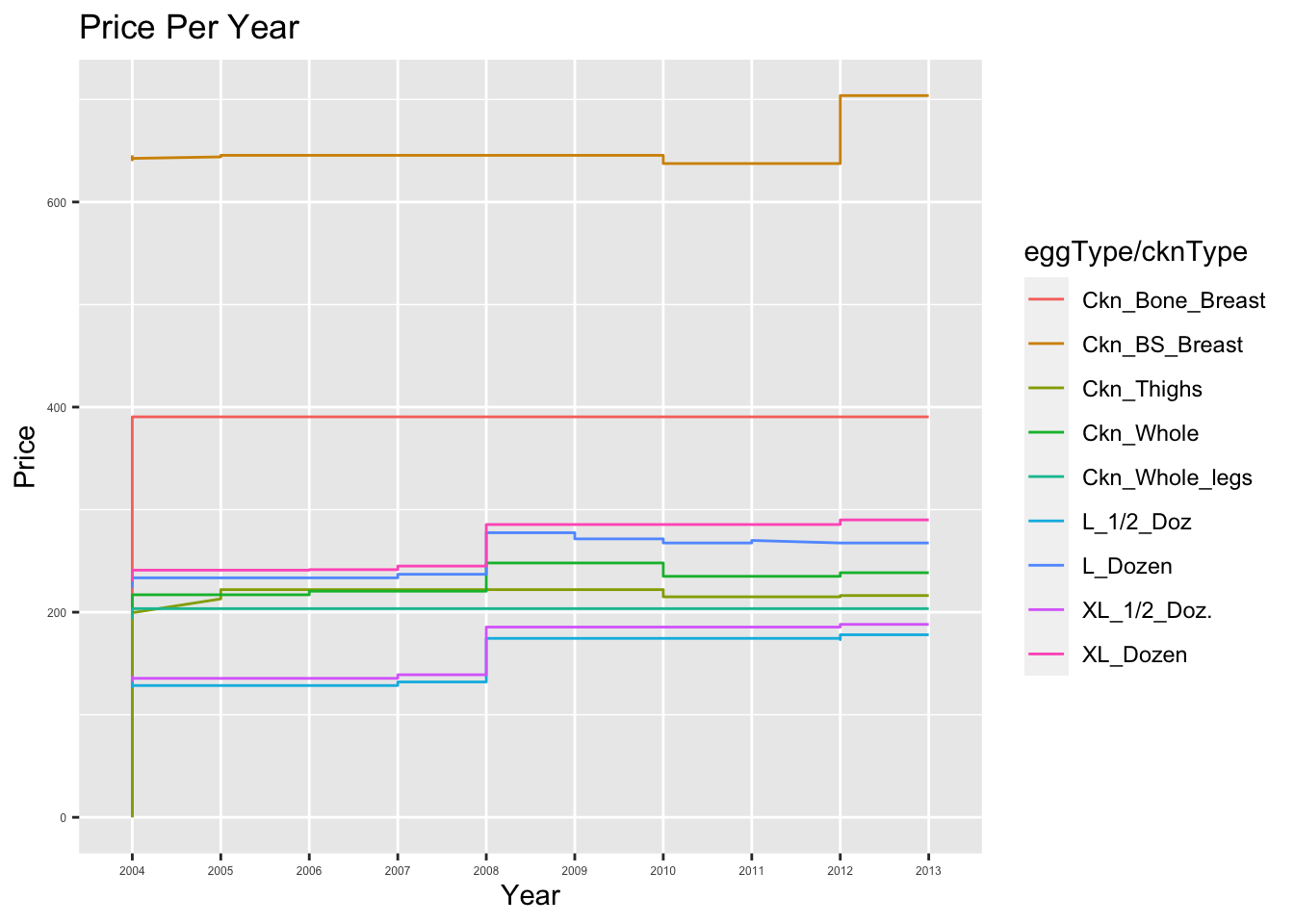

I have included a color coded grab that shows a visual representation of the price per item per year. ## Anticipate the End Result

Code

nrow(eggs_longer)

[1] 1080

Code

ncol(eggs_longer)

[1] 5

The pivoted data has 5 rows and 1080 columns.