Challenge 1 Instructions

Reading in data and creating a post

Code

library(tidyverse)

knitr::opts_chunk$set(echo = TRUE, warning=FALSE, message=FALSE)

Challenge Overview

Today’s challenge is to

1. read in a dataset, and

2. describe the dataset using both words and any supporting information (e.g., tables, etc)

Read in the Data

Read in one (or more) of the following data sets, using the correct R package and command.

• railroad_2012_clean_county.csv ⭐
• birds.csv ⭐⭐
• FAOstat*.csv ⭐⭐
• wild_bird_data.xlsx ⭐⭐⭐
• StateCounty2012.xls ⭐⭐⭐⭐

Find the _data folder, located inside the posts folder. Then you can read in the data, using either one of the readr standard tidy read commands, or a specialized package such as readxl.

Code

# reading data using readr
library(readr)
(data <- read_csv("../posts/_data/railroad_2012_clean_county.csv"))

# A tibble: 2,930 × 3
   state county               total_employees
   <chr> <chr>                          <dbl>
 1 AE    APO                                2
 2 AK    ANCHORAGE                          7
 3 AK    FAIRBANKS NORTH STAR               2
 4 AK    JUNEAU                             3
 5 AK    MATANUSKA-SUSITNA                  2
 6 AK    SITKA                              1
 7 AK    SKAGWAY MUNICIPALITY              88
 8 AL    AUTAUGA                          102
 9 AL    BALDWIN                          143
10 AL    BARBOUR                            1
# … with 2,920 more rows

In case the data it’s not parsed correctly at the column level, we can specify the columns types using spec()

Code

spec(data)

cols(
  state = col_character(),
  county = col_character(),
  total_employees = col_double()
)

Code

data_with_col_types <- read_csv("../posts/_data/railroad_2012_clean_county.csv",
                  col_types = cols(
                  state = col_character(),
                  county = col_character(),
                  total_employees = col_double()
                ))
# printing data
data_with_col_types

# A tibble: 2,930 × 3
   state county               total_employees
   <chr> <chr>                          <dbl>
 1 AE    APO                                2
 2 AK    ANCHORAGE                          7
 3 AK    FAIRBANKS NORTH STAR               2
 4 AK    JUNEAU                             3
 5 AK    MATANUSKA-SUSITNA                  2
 6 AK    SITKA                              1
 7 AK    SKAGWAY MUNICIPALITY              88
 8 AL    AUTAUGA                          102
 9 AL    BALDWIN                          143
10 AL    BARBOUR                            1
# … with 2,920 more rows

Add any comments or documentation as needed. More challenging data sets may require additional code chunks and documentation.

Describe the data

Using a combination of words and results of R commands, can you provide a high level description of the data? Describe as efficiently as possible where/how the data was (likely) gathered, indicate the cases and variables (both the interpretation and any details you deem useful to the reader to fully understand your chosen data).

To know which county has the highest number of employees let’s install a useful library for better data visualization.

Code

install.packages("ggplot2")

Error in contrib.url(repos, "source"): trying to use CRAN without setting a mirror

Code

library(ggplot2)

Let’s check the data.

Code

summary(data)

    state              county          total_employees  
 Length:2930        Length:2930        Min.   :   1.00  
 Class :character   Class :character   1st Qu.:   7.00  
 Mode  :character   Mode  :character   Median :  21.00  
                                       Mean   :  87.18  
                                       3rd Qu.:  65.00  
                                       Max.   :8207.00  

Now let’s use ggplot library to see which state has the highest number of employees regardless the county.

Code

ggplot(data = data, aes(x = state, y = total_employees)) +
  # adding a blue point for each total_employees number
  geom_point(size = 1, color = "blue") + 
  # drawing a straight line to the ponit 
  geom_segment(aes(x = state, xend = state, y = 0, yend = total_employees)) +
  # rotating the the name of the states by 90 degrees
  theme(axis.text.x = element_text(angle = 90, vjust = 0.1)
)

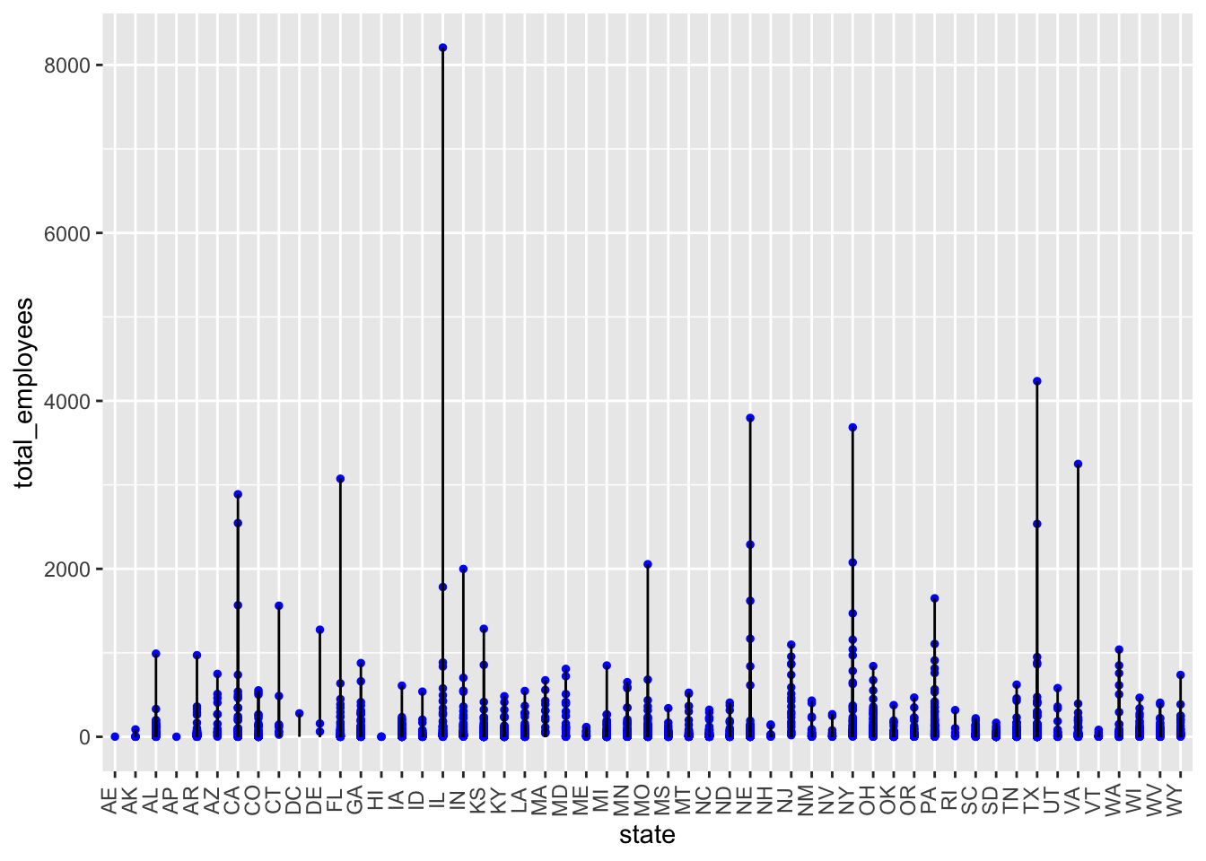
Analysis of the graphic.

The graphic describes the total employees per county for each state regarless the county(later we wil focus on the county). We can observe that Illinois has the highest number of employees. Let’s check more in detail that state.

Filtering the data w have the following data

Code

vars <- c("state")
cond <- c("IL")
data_IL <- data %>%
  filter(
    .data[[vars[[1]]]] == cond[[1]]
  )
data_IL

# A tibble: 103 × 3
   state county    total_employees
   <chr> <chr>               <dbl>
 1 IL    ADAMS                 116
 2 IL    ALEXANDER               2
 3 IL    BOND                   23
 4 IL    BOONE                  44
 5 IL    BROWN                   7
 6 IL    BUREAU                 35
 7 IL    CALHOUN                 4
 8 IL    CARROLL                96
 9 IL    CASS                   66
10 IL    CHAMPAIGN             131
# … with 93 more rows

Let’s plot want we have.

Code

#view(data_IL)
barplot(data_IL$total_employees)

By using the ggplot library, we have more control over how we want to see the data we care about.

Code

ggplot(data = data_IL, aes(x = county, y = total_employees)) +
  geom_point(size = 1, color = "red") +
  geom_segment((aes(x = county, xend = county, y = 0, yend = total_employees))) +
  theme(axis.text.x = element_text(angle = 90, size = 3, vjust = 0.1))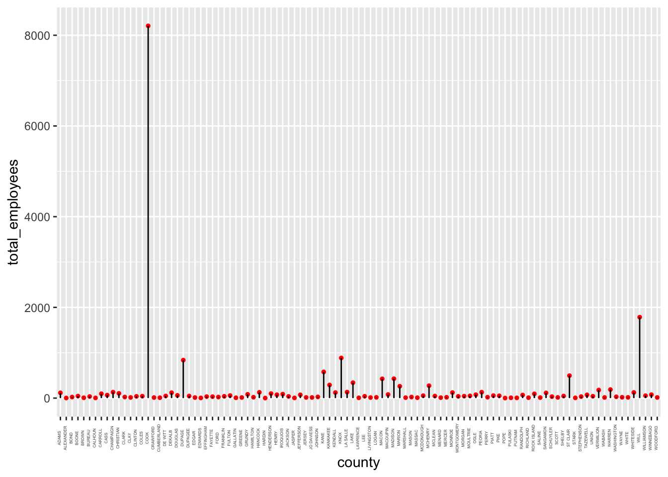

We can conclude that Cook has the highest number of employees in the state of IL.